Using the Oscilloscope

1.1

Plug in the Test & Measurement Device, then start WaveForms and make sure the device is connected.

If no device is connected to the host computer when WaveForms launches, the Device Manager will be launched. Make sure that the device is plugged in and turned on, at which point it will appear in the Device Manager's device list (1). Click on the device in the list to select it, then click the Select button (2) to close the Device Manager.

Note: “DEMO” devices are also listed, which allow the user to use WaveForms and create projects without a physical device.

Note: The Device Manager can be opened by clicking on the “Connected Device” button in the bottom right corner of the screen (3), or by selecting “Device Manager” from the “Settings” menu at the top of the screen.

1.2

Once the Welcome page loads, in the instrument panel at the left side of the window, click on the Scope button to open the Oscilloscope instrument.

1.3

Once the Scope instrument opens, the window contains the data plot (1.) showing captured data, the configuration panel (2.) to right of the plot, and the control toolbar (3.) at the top of the window.

This section walks through setting up the Oscilloscope instrument to capture and analyze a simple waveform.

(NOTE: This guide can be followed using a “Demo” device selected in the WaveForms Device Manager. Doing so allows the user to follow along without having access to an Analog Discovery Studio.)

2.1 Hardware Setup

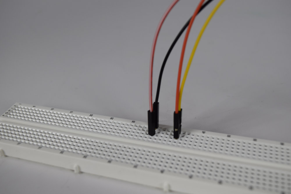
In order to measure a signal with the Scope instrument, there must first be a signal to measure. To this end, step 2.1 of this guide describes setting up a simple loopback circuit that connects the Test & Measurement device's Waveform Generator and Oscilloscope pins.

Connect the test & measurement device's oscilloscope Channel 1 pin (orange wire/circle) to the device's wavegen Channel 1 output pin (yellow wire/circle). For devices that use differential input channels, such as the Analog Discovery Studio with MTE cables, make sure to connect the oscilloscope Channel 1 negative pin (orange wire with white stripes) to the ground pin associated with wavegen Channel 1 (black wire).

2.2 Generating a Signal

With the loopback circuit set up, a signal must now be applied to the analog output pins. WaveForms' Wavegen instrument will be used to accomplish this.

From the Scope instrument, opened in step 1.2, return to WaveForms' Welcome page by clicking on its tab at the top of the screen. In the Welcome tab, open the Wavegen instrument, then click the Run button () in the control bar near the top of the window to begin outputting a signal. With default settings, a 1V amplitude (or 2V_PP) 1 KHz sine wave is applied to the wavegen Channel 1 output pin.

For more detail on how to use the Wavegen instrument, please see the Using the Waveform Generator guide.

Return to the Scope instrument by clicking on its tab in the bar at the top of the screen.

2.3 Begin Capturing Data

Click the Run button in the control bar near the top of the window to begin capturing data on the analog input channels. Captured data will appear in the plot pane as a set of colored lines. The yellow line (labeled 1 in the image to the right) corresponds to the signal captured on analog input Channel 1. The blue line (2) corresponds to the signal captured on analog input Channel 2.

Since analog input Channel 2 was left “floating” (not connected) while making connections in step 2.1, it can be disabled by clicking the Channel 2 checkbox (3) in the configuration panel at the right side of the window.

2.4 Plot Pane Axes

By default, the plot has a vertical range of -2.5V to 2.5V, and a horizontal range of -5ms to 5ms (with respect to the trigger configuration, which is described in section 3.2.

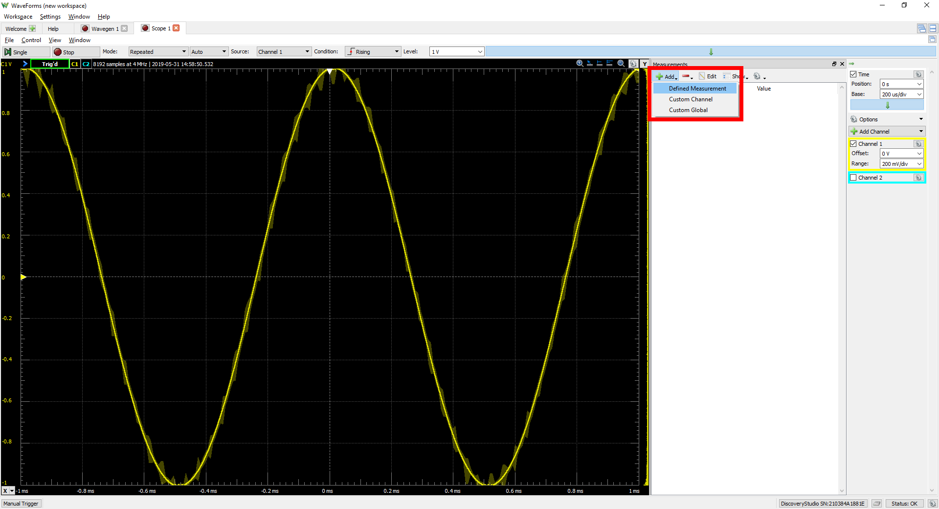
To re-scale the horizontal axis of the plot to show only two periods of the sine wave, change the Base value in the drop-down menu located in the Time box at the top of the configuration panel on the right side (labeled “1” in the image to the right) to “200 us/div”. This value can be set by either selecting a new value from the drop-down (the arrow next to the field), or by clicking into the time base field and manually typing it in (including units and an SI prefix). This specific value represents one hundred microseconds per division (vertical line) on the plot.

To re-scale the vertical axis of the plot, as before, change the Range value in the “Channel 1” box in the configuration panel (labeled “2” in the image to the right). A value of “200 mV/div” will fit the sine wave precisely to fill the entire plot pane.

2.5 Quick Measure Cursors

To take a quick measurement of the period and frequency of the sine wave, click the Quick Measure: Pulse icon() at the top right side of the plot pane. Move the cursor over the sine wave in the plot pane, and observe the values displayed. If the values change too quickly to make out, the capturing of data can be stopped by clicking on the Stop button () in the control bar near the top of the window.

2.6 Measurements

To view calculated values for period, frequency, amplitude, and various others, that may not be available through the Quick Measure cursors, click on the “View” menu in the toolbar just above the Run/Stop button. In the drop-down menu, click on Measurements. This opens a new Measurements pane to the right of the Plot pane.

When opened, the measurements pane does not contain any values. Click on the Add button (), then “Defined Measurement”, to add a new measurement to the list.

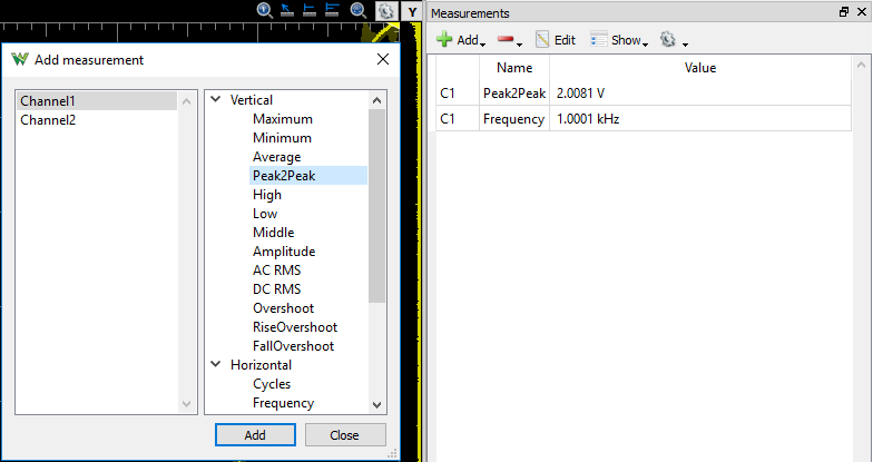
In the popup window, make sure that “Channel 1” is selected in the first list. The second list contains a wide variety of different measurements that can be calculated from data captured from the selected Channel. Expand the “Horizontal” selection, then click on “Frequency” and click the “Add” button at the bottom of the popup window. Under “Vertical”, click on “Peak2Peak”, and then “Add” again. Click “Close”.

Each measurement selected will now be displayed in the Measurements pane. As can be seen, the list of measurements now contains estimates of the frequency and peak-to-peak voltage of the captured signal. As expected, these measurements will be listed as approximately 1 KHz and 2V, respectively.

3.1 Control Buttons

As seen in Section 2, the control bar near the top of the window can be used to stop and start the capturing of data from the analog input pins.

In addition to the Run/Stop button, described above, the Single button can be used to capture a buffer of data based around the first occurrence of a pre-defined trigger. The size of the buffer and when the buffer is captured relative to the trigger event are defined in section 3.3.

The control bar also contains the trigger configuration options, described in the next section.

3.2 Triggers

Immediately next to the Single button are a set of options that can be used to configure oscilloscope triggers. When taking repeated measurements, the plot pane stays centered on these trigger events. As seen above, when the Single button is pressed, a set of data centered on the next trigger event is captured and plotted.

The Mode drop-down allows the user to select what will happen when the Run button is pressed. For descriptions of the available settings, please see the WaveForms reference manual, available through the Help menu in WaveForms, in the menu bar at the top of the screen. The reference manual is also hosted on the Digilent Wiki at this link: WaveForms Reference Manual.

The Source drop-down allows the user to trigger the oscilloscope based on events in other instruments.

The Condition and Level drop-downs allow the user to describe what type of event to trigger on. For example, the configuration Condition = Rising and Level = 1V will generate a trigger event whenever the captured data rises above 1V.

Additional trigger configuration options can be found by clicking on the green down arrow ({learn:instrumentation:tutorials:analog-discovery-studio-oscilloscope:symbol_arrow_down.png?nolink}}) to the right of the level field. Please use the WaveForms Help menu for more information.

By default, the trigger event is centered in the plot. Data captured before and after the trigger can be viewed by modifying Time configuration settings, described in the next section of this guide.

3.3 Time Configuration Group

By default, the Time group in the Configuration panel contains the “Position” and “Base” fields. The Position field centers the plot on the selected time, measured from the trigger. This can be used to view data captured before and after the trigger event. The Base field configures the scale used for the horizontal axis of the plot. Using these two settings can be thought of as “panning” and “zooming” the plot. The time base and position can also be changed with the mouse wheel, and by clicking and dragging the plot pane, respectively.

The Gear button () in the Time group can be used to change the units used in the position and division fields.

Additional time and sampling configuration options can be found by clicking the green down arrow at the bottom of the Time group. For instance, the sample count and rate used when capturing data can be manually configured - it should be noted that doing so also automatically changes the position and base settings. More information on these options can be found through the WaveForms Help menu.

3.4 Channel Configuration Groups

Each input channel of the test & measurement device can be configured via the associated Channel # group in the Configuration panel. By default, each of these groups contains Offset and Range fields. The Offset field is used to set the vertical position of the the captured signal in the plot. The Range field is used to set the scale used for the vertical axis of the plot for that channel. The checkbox next to the channel name can be used to enable or disable that channel, as seen in Step 2.3 of this guide.

Additional options for each channel can be found by clicking on that channel's Gear button. These options can be used to: select the units used for the Offset and Range fields, show or hide the signal's noise band in the chart, modify the channel's attenuation, sampling, and coupling, and others. More information on these options can be found through the WaveForms Help Menu.

3.5 Other Channels

Other types of channels can be added to the plot and Configuration pane through the Add Channel button ().

Math channels can be used to display signals passed through some function. For example, high/low/band pass filters can be applied to signals captured on the analog input channels, and displayed on the plot. Custom functions can be defined using JavaScript syntax.

Reference channels can be used to display custom signals or previously-captured signals (imported from a file) in the plot.

Digital channels can be used to display data captured on the digital input/output channels in a separate pane which appears below the plot. This can be used to view both analog and digital signals at the same time. Digital channels can be also used as inputs to custom math channels in order to display them in the main plot pane. For more information on how digital data can be viewed and used, refer to the Using the Logic Analyzer guide.

3.6 Additional Configuration Options

The Options drop-down above the channel groups contains a set of options that apply to multiple channels at once. For instance, the rate at which the plot is updated can be changed from this menu. For more information on the options available in this menu, please refer to the WaveForms Help menu.

3.7 Chart Pane

The Chart pane displays data captured on the analog input channels. The horizontal axis of the plot represents time before and after the trigger event that initiated the capture. The vertical axis represents the voltage level (or other selected unit, for math and reference channels). Each channel has its own vertical scale, which can be selected by clicking on their identifiers in the top left corner of the plot pane (C1, C2, etc.).

Capture status information can be found next to the channel select buttons, including a state string (Stop / Config / Trig'd). Information about the capture being displayed can be found to the right of the channel select buttons, including the number of samples, sample rate, and a time stamp for when the capture was taken.

Another set of buttons can be found in the upper right corner of the plot panel:

• The Thumbnail button () displays a small version of the entire buffer of data, including indicators for what part of the signal the main plot is currently viewing.
• The three “Quick Measure” tools:
  • Free () measures the distance between two mouse clicks, expressed in time and frequency. It also displays the vertical value and difference of the clicked positions.
  • Vertical () is similar to Free mode but the cursor sticks to signal transitions. The vertical measurement is performed on signal values for each channel.
  • Pulse () places a single vertical cursor showing the time position and the waveform's level at the intersections with the vertical cursor. If the mouse is placed between two peaks of a signal, it measures the pulse-width, period, frequency, and duty cycle of a signal.
• The Show Entire Capture button () zooms the plot all of the way out.

The Gear button next to the previous five buttons can be used to change how the plot is displayed, including adding labels, changing the background between light and dark, displaying all channel scales at once, and others. For more information on these options, refer to the WaveForms Help menu.

The “Y” button and drop-down next to the previous Gear button can be used to add horizontal cursors to the plot. Vertical cursors can be added to the plot using the “X” button and drop-down in the lower left corner of the plot pane.

3.8 File Menu

The File menu at the top of the window provides the ability to create another Scope instrument, as well as to save and load acquisitions and projects.

Saving an acquisition allows the user to load captured data back into WaveForms later. Acquisitions can be loaded into other instruments, as, for example, a signal to be generated by the Wavegen instrument.

Saving a project (with or without any acquisitions) allows the user to close WaveForms without losing any configurations. In addition to this, projects can be shared with others to aid in group projects and guided learning.

Exporting data as an image allows the user to produce a screenshot of the entire Scope tool. Alternatively, captured data can be exported in a variety of different file formats, including CSV, TXT, and TDMS.

3.9 Control Menu

The Control menu at the top of the window provides the same functionality as the Single/Stop/Run buttons, and lists hotkeys that can be used for each.

3.10 View Menu

A wide variety of different view panes can be added to the user interface using the View menu in the toolbar above the Single/Run/Stop buttons. Each pane, once opened, can be closed by clicking the “X” button in the top right corner of its pane. A description of each view in the menu is listed below:

• Add Zoom: Creates an additional plot that can be used to zoom in on particular regions of interest in the signal.
• Add XY: Creates an additional plot with configurable X and Y axes. For instance, two channels can be plotted against one another to create an IV curve diagram.
• FFT: Creates plot to display a Fast Fourier Transform diagram of the captured signals.
• Spectrogram: Creates a spectrogram plot, showing how the frequency components of captured signals change over time.
• Histogram: Creates a plot that displays percentage of time spent by the signal at each voltage level.
• Persistence: Creates a plot that places multiple signal captures on the same plot, with color indicating how often a voltage level is detected at a certain time.
• Data: Creates a chart that exposes raw capture data in a spreadsheet.
• Measurements: As seen in step 2.6 of this guide, can be used to create a list of characteristics of captured signals.
• Logging: Allows the user to log captured data directly to a file, over multiple acquisitions. Includes a scripting interface (JavaScript) with examples.
• Audio: Allows the user to play back captured signals as sound through the host computer's audio output.
• X/Y Cursors: Lists all cursors that have been added to the plot.
• Digital: Exposes some functionality of the Logic Analyzer instrument within the Scope instrument, allowing the user to capture and view data from the digital input/output channels. For more information on capturing and viewing digital signals, please see the Using the Logic Analyzer guide.
• Digital Measurements: Creates a list that can contain features of captured digital signals (frequency, duty cycle, pulse width, etc.).
• Notes: Creates a text editor pane that can be used to document configuration choices, or whatever other information could be useful to remember.