

SPICE simulations are the tool of choice for engineers when designing analog or mixed-signal circuits. Multisim Live from Digilent as browser-based simulator makes this task easy and with the Analog Discovery 3, verifying the results in hardware is not hard as well.
Richard Oed
The big and often discussed question is: “Why should I bother with simulating electronic circuits?” The answer is simple: Because it makes the design process much easier, and it is a great educational tool as well. First of all, simulations save time by reducing the design complexity, as they allow architects of electronic systems to evaluate their development under various conditions. This way, electrical engineers can, for example, optimize the signal-to-noise ratio of their analog front ends through quick iterations without building a new hardware-setup during each step. Simulations also minimize the complexity of tests, as errors can be detected fast because many checks can be performed early on, as can the assessment of failure modes without harming the actual hardware. Testers can spot problems easier, and the insights from data sets created by simulations allow for a speedy troubleshooting process.
And they facilitate an accurate voltage and current waveform analysis through what-if analyses, enabling engineers to understand the behavior of their designs better. This is as well true for analyses in the frequency domain by studying the circuits‘ response to different frequencies or to the analysis of transients – abrupt changes in the input signals. All of this improves the stability and reliability of the circuits. The fine-tuning of component values is also much simplified. Another benefit of simulations is a reduced number of hardware prototypes, as fewer PCB-iterations and purchases of their – sometimes expensive – devices are necessary, saving on costs.
Finally, simulation tools are great for educational purposes. They provide a hands-on interactive learning platform for students in electronics. They can experiment with different circuit variations and comprehend the underlying concepts by visualizing the signals. Furthermore, they can also watch the effects of different components and observe circuit properties, such as gain, resonance, and filtering. In this way, the simulation acts as an intermediary between theoretical principles and real-world applications. By analyzing flawed circuits, students can learn and understand various concepts of fault analysis in a safe environment.
Recognizing the Limitations
Of course, simulations have limits too. First of all, they rely heavily on the accuracy of the underlying algorithms and the validity and precision of the models. Simulation time might also be a problem, as the computational effort increases considerably with complex circuits and a large number of changing parameters. And, since many component properties will be entered manually, there is always the risk that incorrect entries will lead to wrong results. However, engineers who fully exploit the advantages of simulations can create very reliable and cost-effective circuits.
Selecting the Correct Values
Let’s look at an example: Imagine a 10 kHz sine wave containing a sinusoidal component of 75 kHz, which needs to be removed. The simplest way to do so is to use a passive RC low-pass filter with a cutoff frequency (-3 dB frequency) fc of 15 kHz. As a first step, designers must pick the right values for the resistor and the capacitor. To do so, they use the basic formula . Since only the cutoff frequency is known, engineers can freely choose either the value for the resistance R or the capacitance C and calculate the other value. But where to start? There are a couple of points to consider. One of them is to match the components to either the source or the load impedance. A high-impedance source needs a low R, as a high R might cause signal attenuation. A low-impedance load calls for a lower R to avoid influencing the performance of the filter.
There are other factors as well, like power consumption of the system, the thermal noise or the signal-to-noise ratio of low-level signals, which both require a lower R value. There is no one-size-fits-all solution to the problem, so there is some experimentation necessary. And not all values for either C or R are commercially available. So, designing an RC filter is often a compromise, where you begin with one parameter, calculate the second, and balance the result. Let’s say, you will start with a capacitance of 22 nF, which is part of the E3 series of components. Rearranging the equation for R gives a resistance of 482.29 Ω. The closest number in the E3 series would be 470 Ω. Using 22 nF and 470 Ω yields a cutoff frequency of 15.39 kHz, which is fine for our example.
But would this filter work in our case? This is where circuit simulation comes in. Multisim Live from Digilent is an easy-to-use analog and mixed-signal simulator based on the industry-standard SPICE (Simulation Program with Integrated Circuit Emphasis). This tool is free in its basic version.
Multisim Live from Digilent relies on the same simulation technology as National Instrument’s Multisim for desktop. As it is cloud-based, it is platform-independent and can be used without a local installation, as long as the device’s browser is supported. The interface for the schematic entry is like the one of Multisim Desktop and users are able to share the schematics directly through the interface and export them to Multisim 14. To reduce overhead, it comes with a component library, but the number of components accessible depends on the subscription model. The free Basic version allows five components per circuit and four circuits in total.
Simulations are interactive, so you can change parameters of components “on the fly”, with the visually displayed circuit behavior changing immediately. There are six different simulation models available (four for the free version): Interactive, Transient, AC Sweep, DC Sweep, DC Op, and Parameter.
To verify our example, we will first simulate the circuit, confirm it in hardware, and compare the results. In an ideal world, they would be identical.
Setting up the Simulation
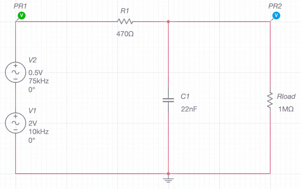
To use Multisim Live, you will need to sign up for an account at https://www.multisim.com. Then go to Circuits → My Circuits and create a new schematic. On the schematic page, you will see the parts toolbar on the left. Add all the components needed: two voltage sources (under Sources), one with a peak voltage VA of 2 V and a frequency of 10 kHz, and one with a VA of 0.5 V and a frequency of 75 kHz. This gives a signal with an amplitude of 2.5 V, containing both frequencies. Add the resistor and the capacitor (under Passive), and a load of 1 MΩ, representing the input impedance of the oscilloscope we want to use later to verify the simulation. Also, add two voltage probes: one before the filter, one after the filter (Figure 2). And you are all set. To create the signal, there is another option as well: the so-called analog behavioral modeling (ABM) sources found under Modelling Blocks where you could describe your signal through an equation. For our case, using two voltage sources is just fine.
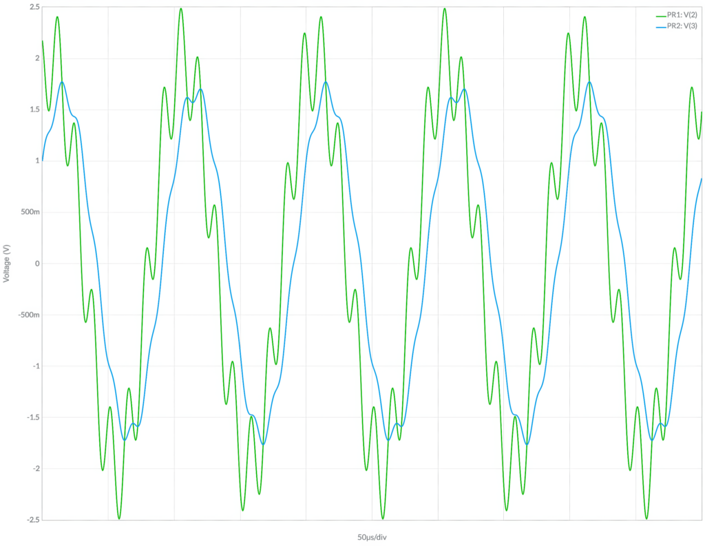
The next step is to run the simulation. To initiate it, go to the Grapher screen and hit the Run button. You will see both voltages plotted on the screen: the voltage after the sources and the voltage after the filter. You will notice that most of the higher frequency components are gone at the curve for Probe 2, demonstrating that the filter works (Figure 3).
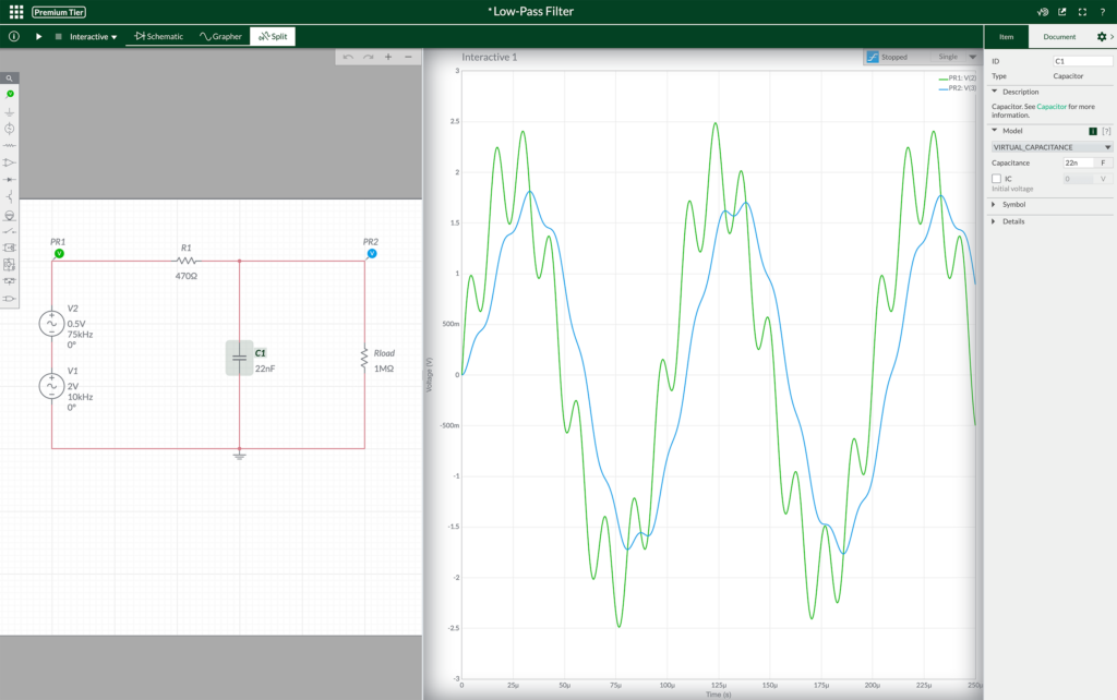
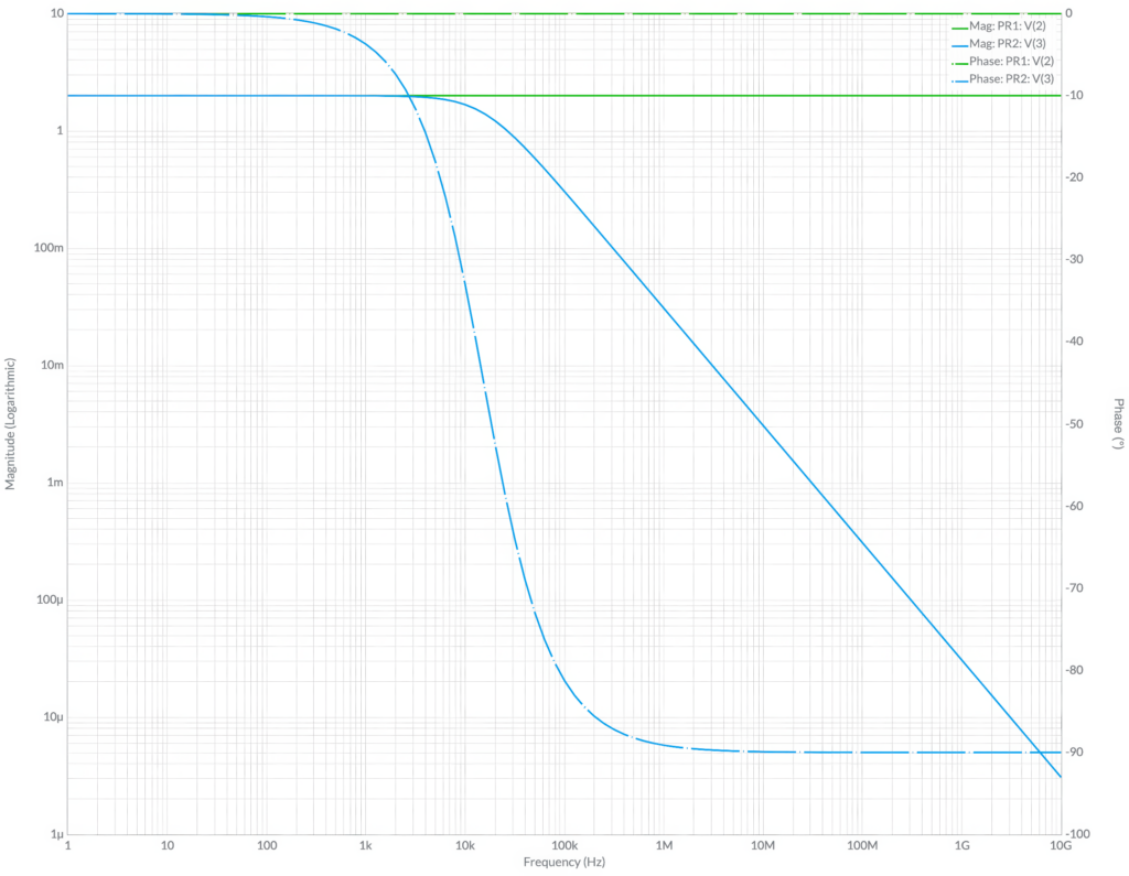
If you want to look closer, press the Stop button and select AC Sweep from the drop-down list beside it. Restart and Multisim Live shows you the logarithmic plot of the magnitudes and phase shifts for the two signals (Figure 4). Go back to Interactive and click on the Split tab. This will bring up the schematic, as well as the graphic display. While the simulation is running, you can modify the values for R or C by double-clicking on the part in the schematic and entering a new value for them in the properties field. This makes it effortless to experiment with different parameters. Please note that you cannot tweak everything while a simulation is ongoing. In this case, stop it, change the value, and restart it. At any time, you can save the graphical view and the schematic by going to the main menu (the nine squares at the left-hand top) and selecting Export.
Verifying the Simulation
But how good is the simulation? As this is a rather simple setup, it is easy to check. A function generator being able to create the source signal, the two discrete components and a two-channel oscilloscope are all what is needed.
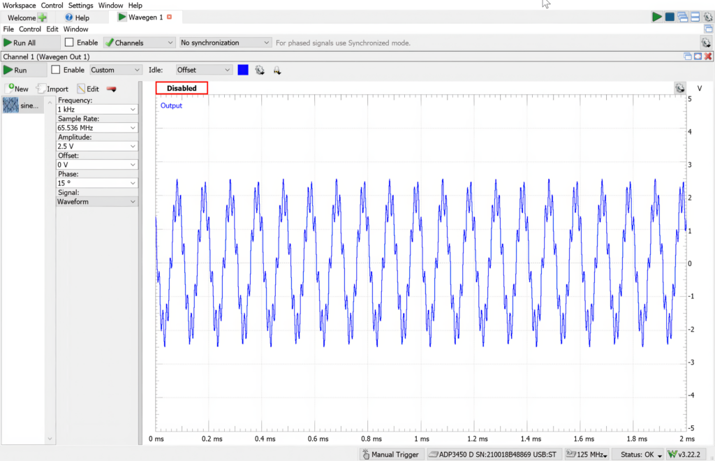
For this example, the author used an ADP3450, Digilent’s 4-channel mixed-signal USB oscilloscope with 125 MS/s, along with the free WaveForms software’s Wavegen instrument as a function generator, to generate a custom waveform described by a mathematical expression. Setting it up requires only a view steps: Call up the instrument, check the Enable box and select Custom from the dropdown-list and finally click on New. Another dialog shows. In the Math tab, you can mathematically describe the waveform you want to create.
In our case, it will comprise two components: the 10 kHz with an amplitude of 2 V and the 75 kHz signal with an amplitude of 0.5 V. Since the resulting amplitude should be 2.5 V, the base sine wave needs to be set to 0.8 of the total, yielding 2.0 V, and the high-frequency part to 0.2, giving a 0.5 V amplitude. This means that you can get the desired signal by entering the following term into the window: 0.8*sin(2*PI*X)+0.2*sin(2*PI*7.5*X), where X refers to the time.
Let X run from 0 to 10 (this leads to 10 periods of the signal), deselect Normalize and hit Generate. You should see the waveform you already know from the simulation. Clicking on Save closes the window. Back in the Wavegen window, make two other changes: set the Frequency to 1 kHz and the Amplitude to 2.5 V. But why 1 kHz? Remember, you created 10 periods, which will now be written to the Wavegen output of the ADP3450 at a rate of 1 kHz, resulting in the desired 10 kHz.
For the oscilloscope to display the voltages, we used an Analog Discovery 3 from Digilent. It not only offers two differential 14-bit channels with a sample rate of up to 125 MS/s per channel and a 30+ MHz bandwidth when using a BNC adapter. It also includes an arbitrary waveform generator, a logic analyzer and a pattern generator for serial interfaces or custom protocols, along with programmable power supplies.
Together with the WaveForms software, additional instruments like the Spectrum, Network, and Impedance analyzers are available as well, as are several other tools.
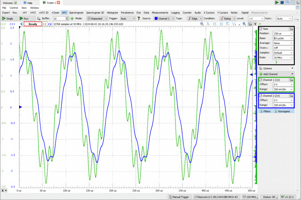
To set up the Analog Discovery 3 as an oscilloscope, open another instance of WaveForms, select Scope, set both channels to a range of 500 mV/div and the time base to 50 µs/div. Connect the ADP3450 and the Analog Discovery 3 to your RC low pass and run both instruments. The oscilloscope graph should now display the unfiltered and the filtered waveform (Figure 6). As a last step, move the zero point for the time to the far left of the screen to make it easier to compare it to the simulation window.
Comparing the Results
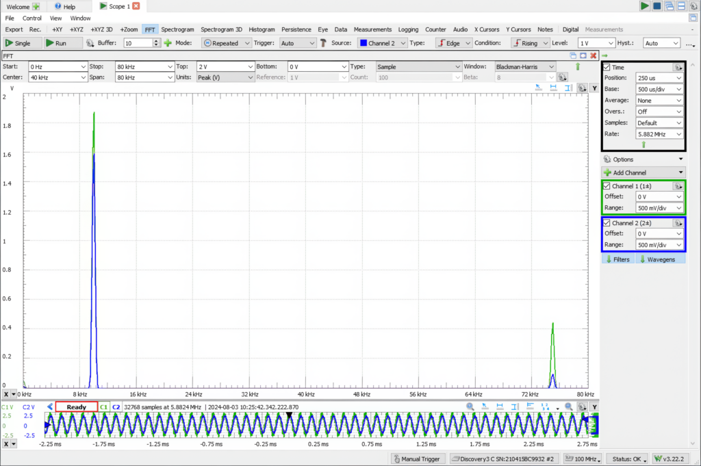
Do they look similar? Yes. But do they look identical? No. Because of real-world effects like additional resistances and capacitances coming from wires, probes, and breadboard, the peak voltages are a bit smaller than in the simulation. Of course, you could build in these parasitic effects into your simulation, but as a first test, this works fine. And if you add an FFT window as well and set the time base to 500 µs/div, you can see that the 75 kHz signal’s amplitude is greatly reduced. This is especially visible if you set the Units to Peak (V) (Figure 7). Now you can fool around and experiment with various parameters, in the simulation but also on the real hardware.
Generally, when you design hardware, there comes a point where you have to build and test the hardware. Without simulation, that point comes very early. But if you use simulation in the concept or design phase, you can start building quite late. Now compare the hardware-only approach with a hybrid approach that uses simulations and hardware later: Which one is easier? Especially, if the design gets very complex.
By harnessing the power of SPICE simulations, engineers can streamline their design process, reduce costs, and improve the reliability of their circuits. Tools like Multisim Live from Digilent make simulation accessible to everyone, from experienced engineers to students.
Ready to take your designs to the next level? Sign up for a Multisim Live account today!