How to Plot the Frequency Response of a Circuit

There are many parameters and behaviors that can be of focus in the analysis of a circuit. One such behavior that I like to nerd out on is the frequency response of a circuit. This means that for some input AC signal applied to a circuit, the response (or output) of that circuit may behave differently for different frequency intervals.

One common way of analyzing frequency response is to consider the “gain” for a given input frequency. Also referred to as the transfer function, gain is typically defined as the ratio of the output voltage to the input voltage: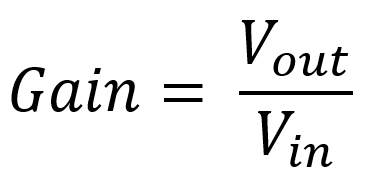     

So, if you’re rockin’ out with your electric guitar plugged into an amplifier, you’re going to experience a lot of gain from your strings to your speakers. Super rad, right?

Kim Thayil of Soundgarden throwing it down with some high gain. Photo from Mesa Boogie at http://mesaboogie.com/amplitudes/2011/August/soundgarden-kim-thayil-san-francisco-ca-july-21-2011.html

Purely resistive circuits generally do not exhibit varying behavior with a change in input frequency, that is, until you get into extremely high frequency circuits. However, energy-storage elements like capacitors and inductors introduce varying behavior that is dependent on an input signal’s frequency. A common application that takes advantage of this varying behavior is a “filter.” Filter circuits generally contain some combination of capacitors and/or inductors. We call them filters because these circuits output voltage only for a defined range of input frequencies, usually with a gain of about 1 and attenuated gain outside that range. For example: if Kim Thayil up there needs more bass frequencies coming out of his speakers for some gnarly riff, the knob he would be turning would be increasing the gain on a low-pass filter (LPF). An LPF allows only lower frequency voltages to the output, attenuating higher frequencies. That’s how Kim cranks up the bass without turning all the other frequencies up, and brings in the thunder!

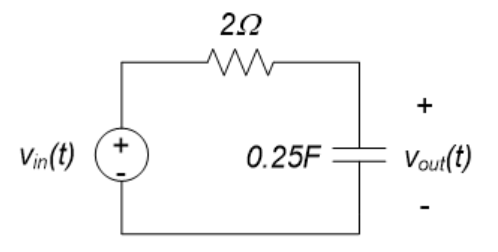
The frequency where attenuation begins is known as the cutoff frequency. For a simple RC circuit, here is Example 11.6 from Digilent’s Real Analog intro to circuit analysis course using our Analog Discovery 2:

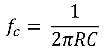
The cutoff frequency in Hertz (cycles per second) can be determined by the formula:

R and C are the resistor and capacitor values of your filter in ohms and farads, respectively. For the example LPF circuit, the cutoff frequency would be about 3Hz, not very practical. Frequencies greater than that will be logarithmically attenuated such that as input frequency approaches infinity, gain approaches zero (no output). Check out Chapter 11 in Digilent’s Real Analog course at https://digilent.com/reference/learn/courses/real-analog-chapter-11/start for more awesome, mathy, and graphical nerd-stuff on frequency response and filtering. You’ll dig it.

So, what’s going on with all these frequencies? How does an LPF really behave? How do we figure this stuff out? There may be two or three routes for you to get to work in the morning, however, one route may be a more efficient use of your valuable time. The same concept applies to circuit analysis techniques and tools.
Let’s say you have designed a filter circuit and need to determine the output response for various input frequencies. There is always the “brute-force” route, which includes: using an oscilloscope to measure input and output voltages to calculate gain and the time difference between peaks to calculate phase for individual input frequencies, plotting the data, then interpolating the results. This process can be exhaustive, will be approximative at best, and just might ruin any fun you were having.

Using the circuit from Example 11.6 with a 1kohm resistor and a 10nF capacitor, we can calculate a theoretical cutoff frequency of about 15.9kHz. Using the Oscilloscope on the Analog Discovery 2, we can measure the gain and phase leading up to this frequency and beyond it, to verify its filtering properties. Using a 1V sinusoidal input, we can start at a low frequency and gradually increase the frequency while adjusting the time axis to get observable and measurable waveforms. Hint: this is the long and tedious way to go about this.

50Hz:

100Hz:

200Hz:

500Hz:

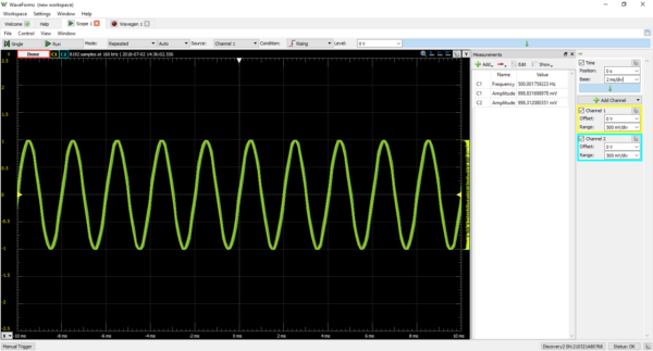
1kHz:

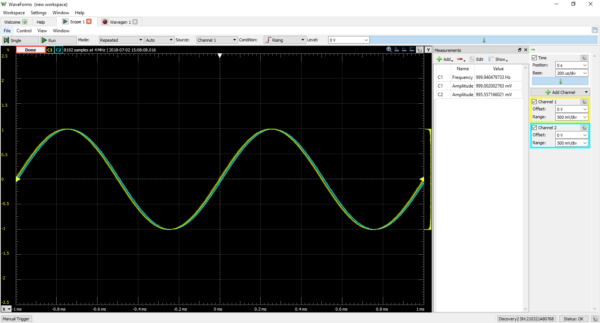
2kHz:

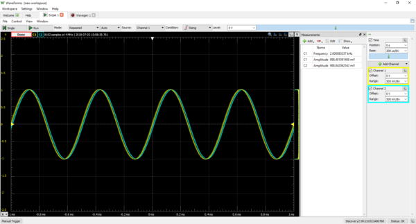
5kHz:

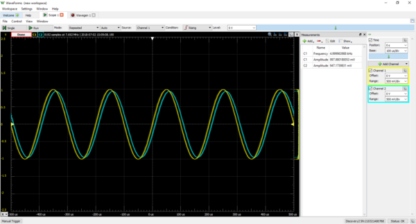
10kHz:

15kHz:

20kHz:

50kHz:

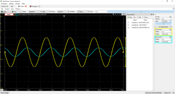
100kHz:

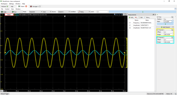
200kHz:

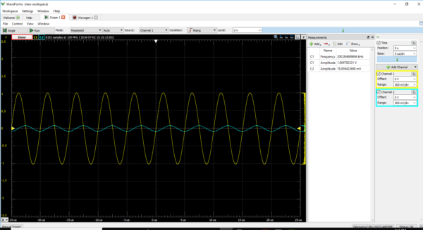
500kHz:

1MHz:

Well, this is certainly a low pass filter with a cutoff frequency around 15kHz. Have fun plotting data and fitting a curve to it.

I had to use a similar approach for my first lab characterizing bi-polar junction transistors (BJTs) and it kind of made me hate my lab professor. It’s good to know that this is an option, but it is about as much fun as getting covered in bees.

Enter Network Analyzer.

The Analog Discovery 2 is loaded with a high-precision, quick response, and customizable Network Analyzer that can plot the gain and phase for your filter over a specified range of frequencies in a matter of seconds.
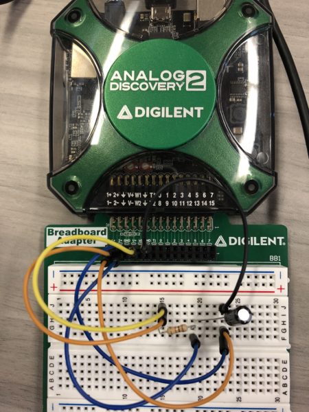
Apply the Arbitrary Waveform Generator and Channel 1 of the oscilloscope to the input of your circuit, and Channel 2 of the oscilloscope to the output.

Using the free, complimentary software, WaveForms, click “Run” in the Network Analyzer window and watch Bode plots of your circuit’s output gain and phase generate as the Analog Discovery 2 sweeps the input frequency. Dang, that’s nice. There is no need to specify any parameters coming from the Wave Generator, although it may be helpful to specify the start and stop frequencies for your input sweep and the sample rate for data precision in the Network Analyzer window.

A cursor can be used to determine the measured cutoff frequency (about 15.5kHz for this circuit, close to our theoretical calculation), phase at a chosen frequency, and more including differential measurements. Nyquist plots and Nichols Plots are also generated for determining the stability of a systematic circuit. The data collected can also be exported for use with other analysis software, like MATLAB.
If you find that your physical circuit is not meeting a design requirement or not responding the way you want it to, make your design modifications and run the Network Analyzer again to determine the new frequency response of your circuit.

Work smart, not hard. A network analyzer is one of many tools in the pocket-sized, USB connecting, multi-function Analog Discovery 2, and is the better solution to learning about frequency response. Unless you are a glutton for punishment.

+1

-1