

Since WaveForms 2015 contains up to eleven analog and digital tools in a single desktop application, it has a lot of options and features. In order to keep the user experience as simple and intuitive as possible, the interface has been designed with simplicity in mind.
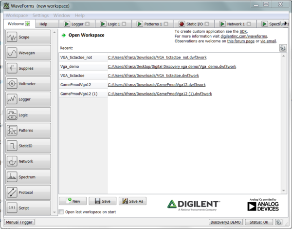
Unfortunately, the vast array of settings and features means that some of these options have to be abstracted. The Quick Start Guide, tool tutorials, and Quick Start Video series all help shed light on the tools themselves and all of the functionality, but sometimes things still get missed. Today I’d like to take a closer look at some of these hidden gems.
Tabs to Windows and Windows to Tabs:
This is one that I only recently discovered myself. When you first open WaveForms, all of the tools default to tabs, but what if you want to have tools in separate windows? This could be useful if you want to view more than one tool at a time without having to switch back and forth between tabs.
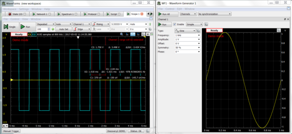
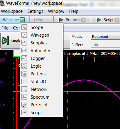
Well, you can! Clicking on the button below will open a tab in a new window, and a window into a tab.
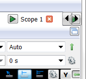
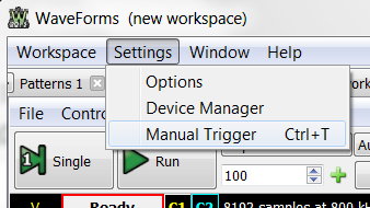
Something to note about this is that if you do this, the manual trigger button will stay in the main window, but don’t despair. There is a keyboard shortcut so you can use the trigger easily from any window.
Saving and Opening a WaveForms Workspace:
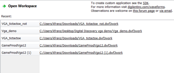
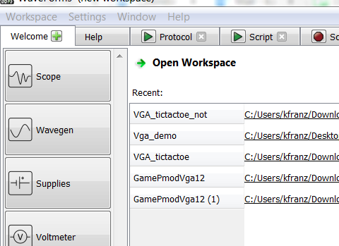
Oftentimes during development, there are tests or measurements that you need to take on a regular basis. And it can be kind of a pain to get all the adjustments and settings just right over and over. In WaveForms, the Waveforms workspace can be saved. This will allow you to save all of your settings and data that is currently open, and the next time you open that workspace, it will be there!
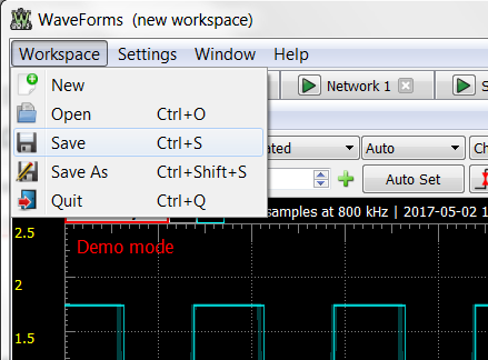
This is also great for demonstrating results, or for working with teams remotely. If you need to send your results to someone else, instead of sending images or having to load the data into another program (by the way, you can also do these things), you can save the workspace and send it to whoever needs the results. This way they can see all your settings and analyze the data in the tool itself.
Green Arrows and Gears:
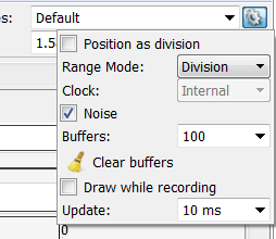
Another thing that’s commonly overlooked is the green arrows and gears.
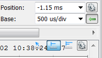
If you can’t find the setting you’re looking for, open a green arrow or gear. The green arrows expand more advanced settings so that the basic functionality isn’t overcomplicated.
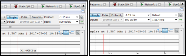
And the gears provide additional settings that aren’t needed by every single user. However, these settings can be extremely useful. I’ll go over some in later hidden gems.
Piece of Paper and Pencil Icon:
Another type of button that will open additional options is the piece of paper and pencil icon.
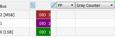
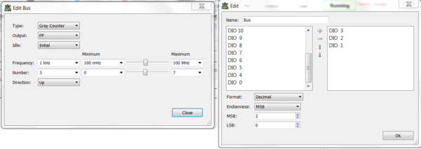
These will open either the parameters or properties windows. For example, in the Logic Analyzer, you see these windows when you add a communication protocol bus initially. But if you want to change the channels or adjust the settings later, just click on the piece of paper and pencil icon.
Plot Labels:
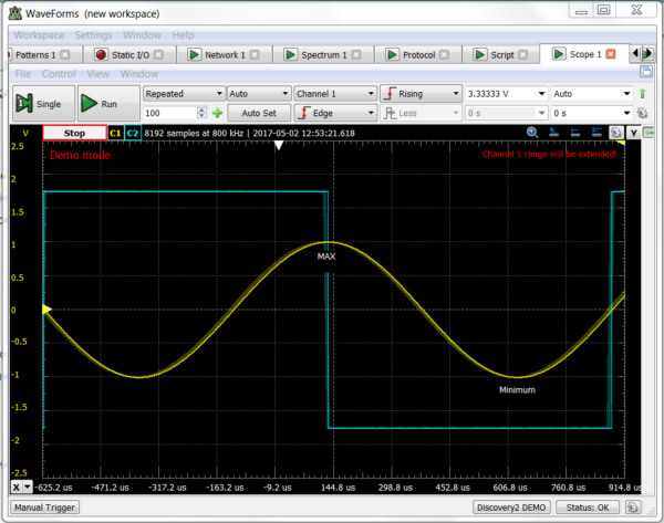
Plot labels are one of the things that you can add from the gear menu in the plot window. You can add a label of text anywhere in your plot window. This can be helpful for labeling specific points, such as the cutoff frequency, and labeling the actual data. This way, when you export the image, the important points are right there on the plot!
Plot Color:
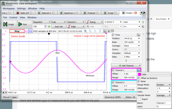
This one is another handy option in the gear menu. Say you’re going to print the image, but boy does that high-contrast black window use a lot of ink. Simply change the plot color to light, and now it’s much more printable.
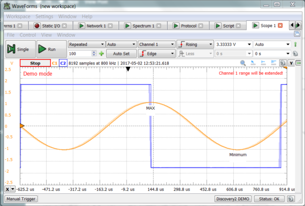
If you change the plot window to light and you don’t feel the traces are clear enough, you can also change the trace colors. Neat!
Measurements:
This is another one that I had no idea existed until recently. In the plot window within the gear menu, there are several types of measurements you can take in the plot.
Free measurements takes a measurement between any two mouse clicks.
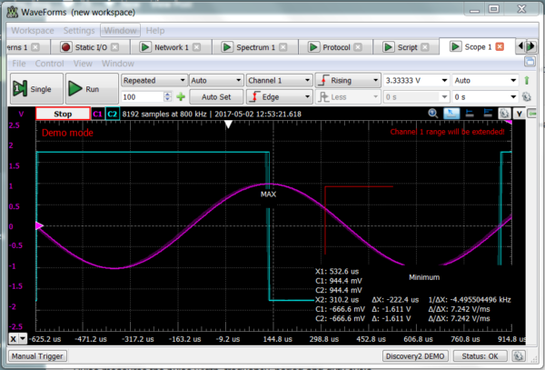
Vertical works the same as free, except it sticks to the signals.
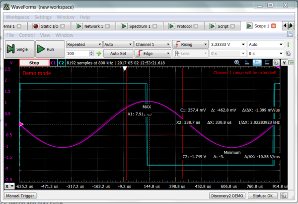
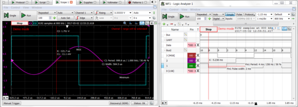
Pulse measures the pulse width, frequency, period, and duty cycle.
Cursors:
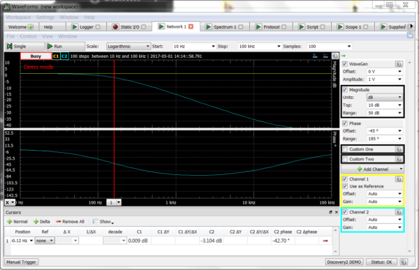
Cursors can be added from the cursor window or from the x or y symbols on the plot window. You can add x cursors and y cursors in the Oscilloscope and x cursors in the Logic Analyzer, Network Analyzer, and Spectrum Analyzer. A single cursor will show positions on the traces.
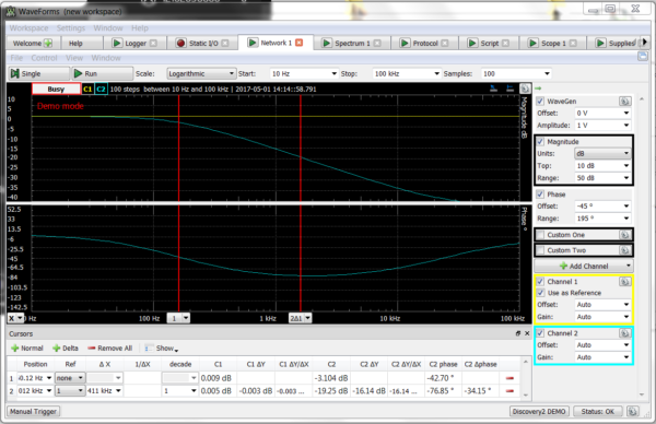
A delta cursor will show the differences between the two traces in a variety of units depending on the tool.
The view menu:
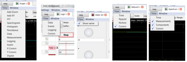
The view menu at first inspection might seem like it would just give you different options on how to view the data, and that would be kind of correct. It does give you different ways to view the data, but not in the traditional way. It will instead give you different types of plots and measurement tools. The options are different depending on the tool.
Data Export:
This one might not be so secret, but it is slightly hidden in a menu, so I figure it’s worth mentioning. You can export data from any tool. You can export the plot window as an image or export the data itself.
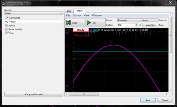
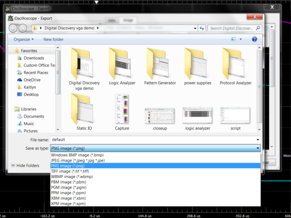
You can export as most types of image formats and the data as a text, CSV, or tdms file.
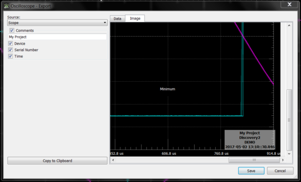
If you export as an image, you can also add a name, device, time, and date stamp.
Dropdowns also allow text editing:
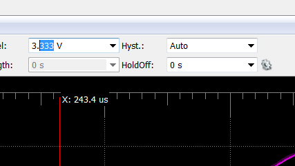
Most of the settings where you choose a value are shown as a dropdown where you can select values in set increments. In addition to being able to select those set values, you can enter custom values. This way, if you know the value you want, you can type the value in instead of searching for it, and add more exact values when needed.
“Knob-like” functionality:
Another feature of those dropdowns is the “knob-like” functionality. If you have a scroll wheel on your mouse, you can use that to increase and decrease the values in a dropdown similar to how a knob works. If you don’t have a mouse with a wheel, you can use the touchpad in a similar manner. Just use two fingers and drag up and down to scroll.
The small icons are actually buttons:
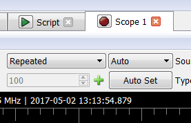
When you have the tools and navigation bar set as tabs, each tab has a label and a small icon indicating the status of that tab. That icon is actually a button! You can use it to run or stop the tool and use it to select a tool in the navigation bar.
The Help Tab:
When you open WaveForms, one of the tabs that automatically opens is the help tab. The help tab contains documentation on each of the tools and definitions of all the buttons and options.
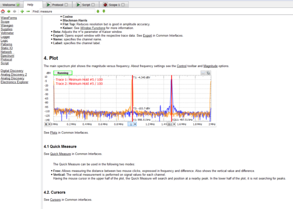
This is a great place to look if you get stuck because it is built directly into the tool. And of course, if you need more help than the help tab can provide, you are more than welcome to look in the resource center. There you’ll find tutorials, community projects, and a getting started guide.
The Device Manager:
When you first open up WaveForms, you’ll see the device manager.
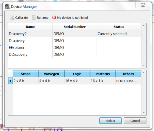
Once the device is selected and connected, it disappears and tends to get forgotten. The device manager does more than just allow you to select the device. You can also name your device, calibrate your device, troubleshoot connections, and allocate resources to the tools.
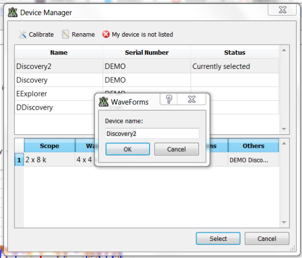
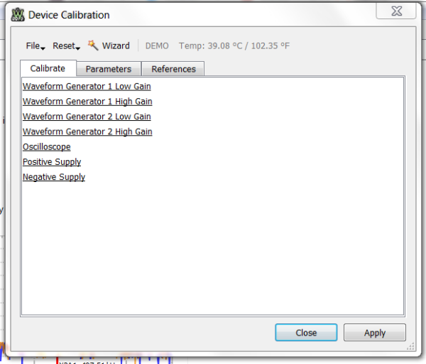
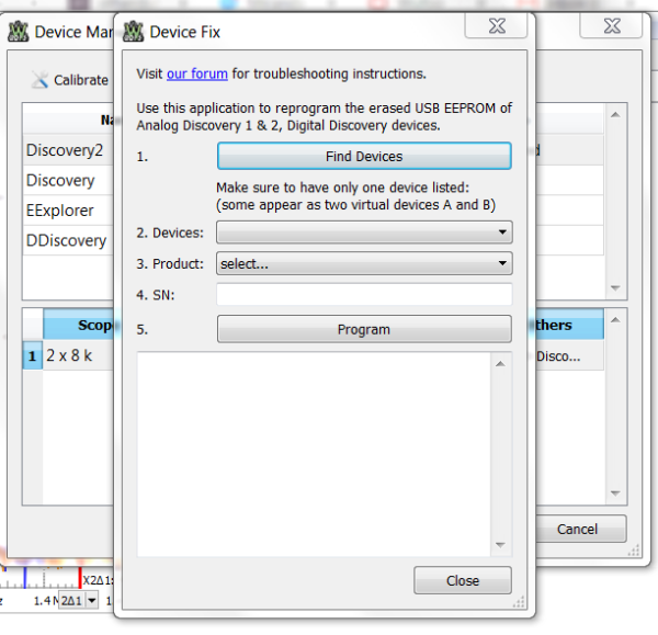
If you don’t care to get to know the device manager, that’s fine. All instrumentation devices are factory calibrated and have default settings.
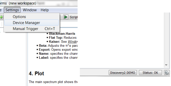
You can access the device manager through the leftmost button in the bottom left of the screen, or in the settings menu.
System Monitor:
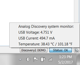
Next to the button that opens the device manager is the system monitor, which will tell you the status of the device. If you click on it, you’ll be able to see the Analog Discovery 2 USB current, USB voltage and temperature, the Digital Discovery USB current, USB voltage, user current and user voltage, and the state of the power switch for the Electronics Explorer Board.
The Forum:
This is not really hidden, but it is still a gem! If you run into any problem you can’t solve, or you have suggestions, post on the Digilent forum. Your input is always welcome.
That concludes the Hidden Gems series. If you have found any hidden gems yourself that I missed, comment below! And of course, make sure to check out WaveForms, free to download, and keep following the blog.


