

Introducing JupyterLab
JupyterLab is a relatively new tool. It is an open-source development environment (IDE) for working with Jupyter notebooks. Notebooks are primarily used to combine program code, code results, documentation or discussion, and visualizations in one file. They can execute code in individual cells, making interacting with the code and its results easier. JupyterLab can open more than one notebook in separate tabs, like a web browser with tabs pages pointing to various sites. Upon startup, it reads a workspace file to know which notebooks to load. This brief article introduces Jupyter Lab and demonstrates how to control a USB-201 and acquire and display actual analog data.
JupyterLab can be thought of as an enhanced version of Jupyter Notebook, but with more features:
- User Interface: It presents a flexible interface that helps to organize your work better
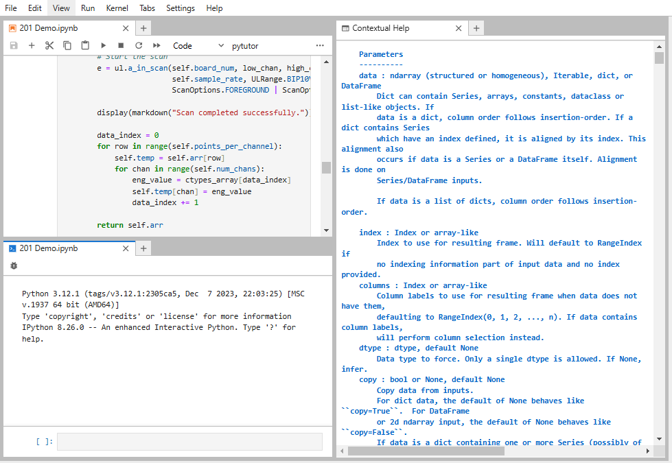
- File Management: It includes a file explorer to open notebooks, a Python terminal, contextual help, and more.
- More: Jupyter Lab has an advanced extension system, much more than Jupyter Notebook, that allows users to customize its functionality. Extensions for Google Drive and GitHub exist that allow for improved collaboration.
Whereas a Jupyter Notebook is straightforward. It is a single notebook file containing separate cells for Python code, text output, and information display.
What sets JupyterLab apart from Notebook?
Jupyter Lab is designed to enhance workflows, as in data science applications. Its multi-document interface allows users to manage notebooks, text files, terminals, and consoles in a single workspace. This capability increases productivity by enabling multitasking and better organization. When adding a new notebook, you can choose between Python 3, a Python console, a power shell terminal, Text, code, HTML, or Markdown. Selecting Python 3 will provide individual cells, which we can use to execute code and display HTML or Markdown text as comments, titles, notes, or whatever. For instance, the Display’s Markdown, Math, and LaTex interfaces can be used for documentation.
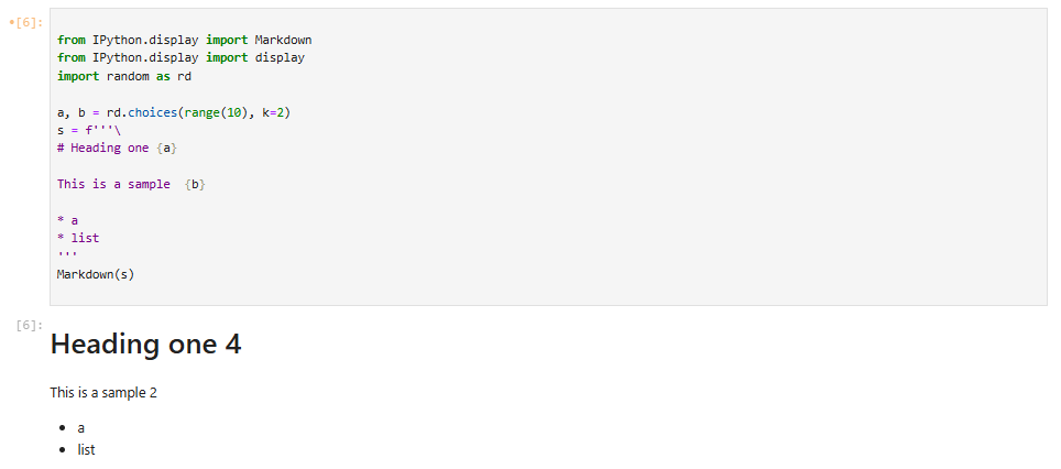
Displaying Markdown language from within a code cell:
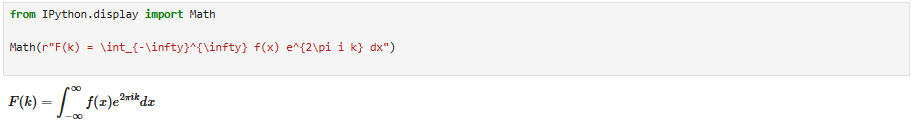
Displaying Math from within a code cell:
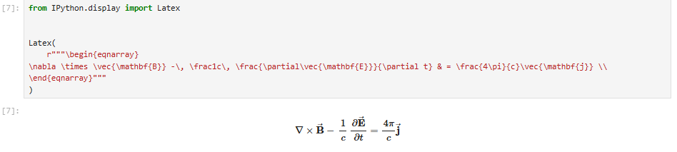
Display LaTex from within a code cell:
Advantages of Using JupyterLab
JupyterLab’s appeal lies in its ability to combine documentation, code, and live results. Its user-friendly interface makes it accessible to beginners, while its advanced features cater to experienced developers and researchers. It is a preferred tool in fields such as Data Science.
Interactivity is another distinctive feature. The ability to execute code in chunks and observe immediate outputs encourages an iterative approach to problem-solving. This hands-on methodology is particularly effective for refining code algorithms or running multiple experiments.
Moreover, JupyterLab’s cross-platform compatibility ensures it can run on various operating systems, including Windows, macOS, and Linux. This universality, coupled with its browser-based nature, eliminates installation hurdles and enhances accessibility.
Applications
JupyterLab’s versatility extends to numerous disciplines. In data science and machine learning, it is a comprehensive tool for preprocessing, modeling, and visualization.
JupyterLab is a valuable tool for Researchers who simulate and analyze experimental data. It can be used in education to create teaching materials, enriching the learning experience.
Analysts rely on JupyterLab to generate results, prepare reports, and build dashboards. Software developers use it to prototype algorithms and document workflows, making it a valuable addition to their toolkit.
Installing Jupyter Lab
Installing JupyterLab is super easy. First, start a command console (CMD) or terminal. Next, upgrade pip by entering the command below. If it fails, ensure that you have installed Python.
C:\users\name> python –m pip install –upgrade pip
Now install Jupyter Lab as follows:
C:\users\name> pip install jupyterlab
To start Jupyter Lab, enter the following:
C:\users\name> jupyter lab
The remaining discussion is about acquiring data from an MCC USB-201 device. For this, I created a Python class to configure an acquisition for a USB-201 (available on Digilent.com). Creating the class object attempts to contact the USB-201, and if found, it establishes communication and sets the sample rate and number of samples per channel. The get data method returns a 2D array (rows, columns), and there is a routine to plot the data. Matplotlib and IPython’s Display module display the 2D array as a plot and list the array in a row-column fashion.
This a simple acquisition. The channel numbers are fixed to be channel 0 through channel 3. The limitation is 2000 samples per channel, and it uses the FOREGROUND mode, which blocks the code until the desired number of samples is returned. However, although the FOREGROUND mode blocks the code, the notebook will highlight the next cell as if it has finished. This can be demonstrated by configuring an acquisition requiring several seconds or more to finish.
The entire notebook is available on GitHub, here: USB-201-Jupyter/USB-201-Demo.ipynb at main · Digilent/USB-201-Jupyter. The following images demonstrate acquiring data from a USB-201.
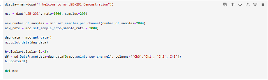
My notebook’s first cell defines my class object, which has the code to acquire data from the USB-201. The structure is as follows:
Class daq:
    __init__
        Initializes internal variables
        Calls open_device
    __del__
        Closes the device and frees allocated memory
    open_device(name)
    set_samples_per_channel(samples)
    set_sample_rate(rate)
    array = get_data()
    plot_data(array)
The first line, mcc = daq(“USB-201”, rate=1000, samples=200), creates the class object and sets the sample rate and the number of samples per channel.
Next, we can use class methods to update the number of samples per channel and sample rate.
new_number_of_samples = mcc.set_samples_per_channel(number of samples = 2000)
new_rate = mcc.set_sample_rate(sample_rate = 2000)
Next, we grab a 2D array containing the acquisition’s data using the following command:
daq_data = mcc.get_data()
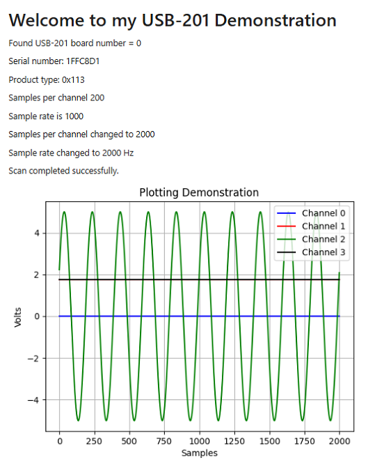
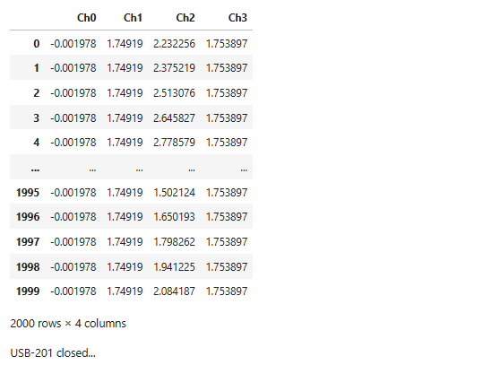
daq_data is passed to the plot method, which plots the data. The IPython Display module is also used to display the data nicely. You can run the acquisition multiple times while mcc is valid. For instance, using a loop to collect additional data. Before leaving the cell, destroy the mcc object to close the device and free the allocated memory.
JupyterLab Widgets
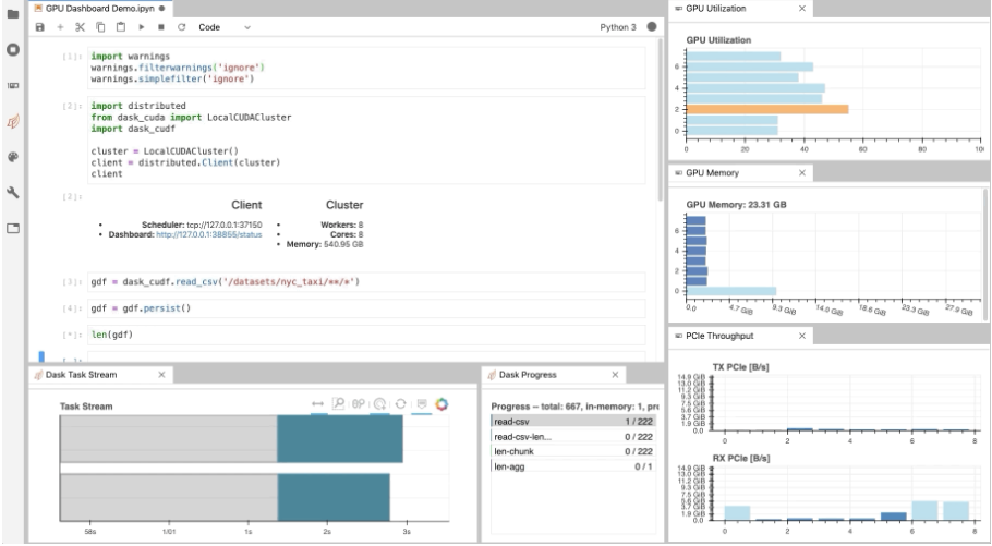
One of JupyterLab’s standout features is its support for interactive widgets. These widgets provide real-time data manipulation and visualization. These included controls, such as a text area, text box, select and multi-select controls, checkbox, sliders, tab panels, grid layout, etc. The display below is a dashboard example that visualizes live data. Jupyter Lab’s ability to customize with Extensions and Widgets ensures it remains relevant across diverse use cases
To exit JupyterLab, under the File menu, select Shutdown.
Conclusion
If it involves Data Science algorithms, scientific research, or education, JupyterLab will help. Its Extensions and Widgets make it a more robust interface than its initial appearance. It opens a new door to documenting scientific research, code algorithms, and the results they produce.