

Consider Dash if you’ve ever wanted to create a web browser application using Python. With Dash, you don’t need to be good at using JavaScript, great at Cascading Style Sheets (CSS), and excellent at the Hypertext Markup Language (HTML). An application is structured like HTML, but with Python. Interaction with the outside world is handled with callback functions. In the truest sense, the application is stateless, meaning no data is passed between functions or maintained locally. Each time it runs, it has no memory of previous runs. Stateless applications tend to be simpler in design, have faster execution, and use fewer resources.
In this article, I will discuss how a stateless web application can be used as a front end to a program, how callbacks work, and what triggers them. To understand all this, I’ve simplified the web server Python example included with the MCC Daqhat data acquisition boards. I’ve converted the example to show simulated data as sine waves instead of vibration data from an MCC 172 or sensor data from an MCC 128.
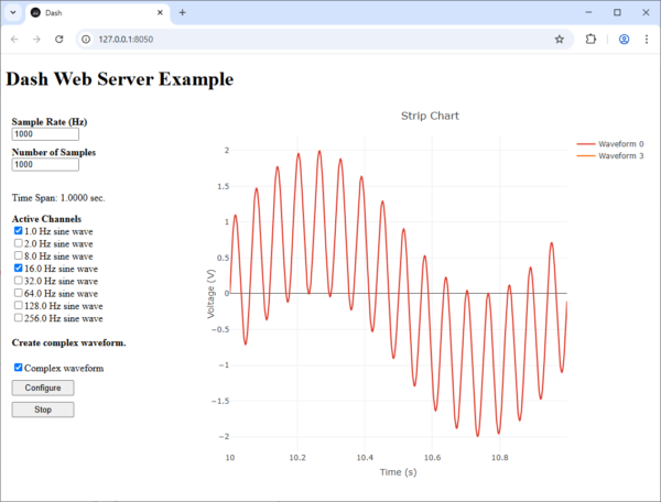
The program consists of two textboxes, a list of checkboxes, two buttons, and a single graph to display the data. There is also a hidden message field to display an error message if a mistake is made, like not checking at least one waveform box. The two text boxes are for Sample Rate (Hz) and Number of Samples. The Number of Samples divided by the Sample Rate (Hz) sets the duration of the X-axis, in seconds. These two parameters are also used to calculate the tick interval of a timer. The timer, when running, triggers certain callbacks to update the graph and give the appearance of a continuous sine wave.
The program begins by launching an HTML web page. Instead of using local variables and lists, it stores data using HTML elements. For instance, the chartData container stores the data in the graph. It is initialized using the default Number of Samples and Sample Rate to have 1000 null values and an X-axis time of one second.
html.Div(
    id='chartData',
    style={'display': 'none'},
    children=init_chart_data(1, 1000, 1000)
),
Like a state machine, this program uses four states for control: idle, configured, running, and error, which are stored in the status element.
html.Div(
    id='status',
    style={'display': 'none'}
),
Pressing the Configuration button updates the status element, which triggers any callback using status as an Input() in the callback function signature. One of those callbacks is called disable_channel_checkboxes. It cycles through all the checkboxes to disable and grey them out. The Output() in the function signature is its return variable. It returns the channelSelections list, which updates the display.
@app.callback(
    Output('channelSelections', 'options'),
    [Input('status', 'children')]
)
def disable_channel_checkboxes(acq_state):

    num_of_checkboxes = 8
    frequencies = [1.0, 2.0, 8.0, 16.0, 32.0, 64.0, 128.0, 256.0]  # Hz
    options = []
    for channel in range(num_of_checkboxes):
        label = str(frequencies[channel]) +' Hz sine wave '
        disabled = False
        if acq_state == 'configured' or acq_state == 'running':
            disabled = True
        options.append({'label': label, 'value': channel, 'disabled': disabled})
    return options
The disable_channel_checkboxes callback inputs status and is triggered by a status change. State() can be used to avoid triggering unnecessary callbacks. In the function start_stop_click, Input() is used only for the two buttons. The rest of the function parameters use State() to avoid triggering unnecessary callbacks. For more on callback, please refer to: https://dash.plotly.com/basic-callbacks
@app.callback(
    Output('status', 'children'),
    [Input('startButton', 'n_clicks'),
     Input('stopButton', 'n_clicks')],
    [State('startButton', 'children'),
     State('channelSelections', 'value'),
     State('sampleRate', 'value'),
     State('numberOfSamples', 'value')]
)
def start_stop_click(btn1, btn2, btn1_label, active_channels,
                     sample_rate, number_of_samples):

    button_clicked = ctx.triggered_id
    output = 'idle'
    if btn1 is not None and btn1 > 0:
        if button_clicked == 'startButton' and btn1_label == 'Configure':
            if number_of_samples is not None and sample_rate is not None and active_channels:
                if (999 < number_of_samples <= 10000) and (999 < sample_rate <= 10000):
                     output = 'configured' else: output = 'error' else: output = 'error'
                elif button_clicked == 'startButton' and btn1_label == 'Start':
                    output = 'running' if btn2 is not None and btn2 > 0:
        if button_clicked == 'stopButton':
            output = 'idle'

    return output
The timer element is the heartbeat. For instance, the update_strip_chart_data callback inputs it to refresh the chartData element continuously on each tick of the timer. When idle, an interval of 1 day is used to disable the timer. When running, start_stop_click artificially restricts Number of Samples and Sample Rate to a range between 1000 and 10000, or a timer interval between 0.1 and 10.0 seconds. When update_timer_interval detects running as the status, it recalculates the timer interval based on the Number of Samples and Sample Rate.
dcc.Interval(
      id='timer',
      interval=1000 * 60 * 60 * 24,
      n_intervals=0
),
When data is available, the update_strip_chart_data callback loads the new data into chartData, not the graph. However, changing chartData triggers the update_strip_chart callback, which transfers the chartData data into the graph you see. Because the timer is essentially turned off at start, update_strip_chart_data must input the status so that it can be called when the user presses the Start button, which changes the status. From there, the timer takes over.
@app.callback(
    Output('chartData', 'children'),
    [Input('timer', 'n_intervals'),
     Input('status', 'children')],
    [State('chartData', 'children'),
     State('numberOfSamples', 'value'),
     State('sampleRate', 'value'),
     State('channelSelections', 'value'),
     State('sumChannels', 'value')],
    #prevent_initial_call=True
)
def update_strip_chart_data(_n_intervals, acq_state, chart_data_json_str,
                            number_of_samples, sample_rate, active_channels, make_complex):

    updated_chart_data = chart_data_json_str
    samples_to_display = int(number_of_samples)
    num_channels = len(active_channels)

    if acq_state == 'running':
        chart_data = json.loads(chart_data_json_str)

        frequencies = [1.0, 2.0, 8.0, 16.0, 32.0, 64.0, 128.0, 256.0]  # Hz

        duration = float(number_of_samples / sample_rate)
        start_time = duration * _n_intervals

        t = np.linspace(start_time, start_time + duration, int(sample_rate * duration), endpoint=False)

        sine_waves = np.array([np.sin(2 * np.pi * f * t) for f in frequencies])

        data = sine_waves[active_channels]if len(make_complex) > 1:
            temp = sum(data)
            num_channels = 1
            sample_count = add_samples_to_data(samples_to_display, num_channels,
                                               chart_data, temp.flatten(), sample_rate)
        else:

            sample_count = add_samples_to_data(samples_to_display, num_channels,
                                               chart_data, data.T.flatten(), sample_rate)

        # Update the total sample count.
        chart_data['sample_count'] = sample_count

        updated_chart_data = json.dumps(chart_data)

    elif acq_state == 'configured':
        # Clear the data in the strip chart when Ready is clicked.
        updated_chart_data = init_chart_data(num_channels, int(number_of_samples), sample_rate)

    return updated_chart_data
When the status equals ‘running’, update_strip_chart_data and update_strip_chart are called one after the other..
@app.callback(
    Output('stripChart', 'figure'),
    [Input('chartData', 'children')],
    [State('channelSelections', 'value')]
)
def update_strip_chart(chart_data_json_str, active_channels):

    data = []
    xaxis_range = [0, 1000]
    chart_data = json.loads(chart_data_json_str)
    if 'samples' in chart_data and chart_data['samples']:
        xaxis_range = [min(chart_data['samples']), max(chart_data['samples'])]

    if 'data' in chart_data:
        data = chart_data['data']

    plot_data = []
    colors = ['#DD3222', '#FFC000', '#3482CB', '#FF6A00',
              '#75B54A', '#808080', '#6E1911', '#806000']
    # Update the serie data for each active channel.
    for chan_idx, channel in enumerate(active_channels):
        scatter_serie = go.Scatter(
            x=list(chart_data['samples']),
            y=list(data[chan_idx]),
            name='Waveform {0:d}'.format(channel),
            marker={'color': colors[channel]}
        )
        plot_data.append(scatter_serie)

    figure = {
        'data': plot_data,
        'layout': go.Layout(
            xaxis=dict(title='Time (s)', range=xaxis_range),
            yaxis=dict(title='Voltage (V)'),
            margin={'l': 40, 'r': 40, 't': 50, 'b': 40, 'pad': 0},
            showlegend=True,
            title='Strip Chart'
        )
    }

    return figure
This example is available for download:https://github.com/JRYS/DashServer
To run the example, you must have Dash installed. Fortunately, installing it could not be easier. In a terminal, enter the following:
pip install dash
This also adds the Plotly graph objects library.
The example, when run in Jupyter Notebook, should start automatically. However, in a Python IDE, you must use the provided IP address (127.0.0.1:8050) entered into your browser’s address bar to start it. Most of the time, you can click the IP shown in the debug window to launch it.