Getting Started with LabVIEW and a Digilent Discovery Device

The following guide presents how to install and use the Digilent WaveForms VIs LabVIEW package, to control Digilent Test and Measurement devices. Demos for controlling the Power Supply, the Digital I/O lines, the Waveform Generator, and the Oscilloscope instruments can be found in the Examples section of this document.

Note: If a Test and Measurement device without analog input and/or output channels (Digital Discovery), or without variable power supplies (Analog Discovery) is selected, certain examples in this guide will not work.

Note: The latest installers for WaveForms can be downloaded Digilent's hosting area here and the set up process is found in the WaveForms Getting Started Guide. By installing WaveForms, the Digilent WaveForms Runtime will be installed, which is needed by the WaveForms VIs.

Note: To download LabVIEW, an NI account is needed. Alternatively, LabVIEW Community can be downloaded from LabVIEW Community and a getting started guide can be found at LabVIEW Community Getting Started. LabVIEW's Add-On Tool, VI Package Manager (VIPM), is used in this guide. Installation of VIPM is mentioned in the guide.

If you're looking for LabVIEW support for Measurement Computing (MCC) and Data Translation (DT) devices, check out these resource centers: Universal Library for NI LabVIEW™, LV-Link Software Interface for NI LabVIEW.

What to do if the VI Package Manager is not installed?

If the VI Package Manager option is not listed under the Tools menu, select the Find LabVIEW Add-ons option.

The NI Tools Network web page will open. Enter VI Package Manager in the search field. Select the JKI VI Package Manager Download from the search results.

Click on DOWNLOAD and proceed to install the VI Package Manager (VIPM) application onto the target Windows system. Close LabVIEW if open and then launch the VIPM application. (Continue with the next step in this guide.)

What to do if you get a Batch Process Error?

If prompted with a VIPM - Batch Process Error, click the OK button.

Next, click the Finish button and restart LabVIEW.

Once back into LabVIEW, click on Tools from the top menu and then select Options.

In the Options window, select VI Server and then scroll down on the right side until you reach Machine Access. Enter your system name in the Machine name/address field and then click the Add button to add the name to the Machine Access List. Afterwards, click the OK button.

Note: Use Windows System Information to determine your computer's system name.

Power Supply Example

Download and unzip the provided example file variable_power_supply_v2.zip then double click on it to open it with LabVIEW. All the instruments used in the example can be used in your own VI, play around and see what else you can create.

To use the Power Supply instrument within LabVIEW, the following subvis are available in the Measurement I/O → Digilent WF VIs → Power Supply container:

• Initialize: allows the user to select the Digilent Test and Measurement device and sends the device handler to the other power supply subvis.
• Voltage: is used to set the voltage level and the current limit for channels V+, V- or VIO.
• Enable: enables/disables the power supply channels.
• Close: Closes the instrument when the program is terminated, making it available for other software (no instrument can be controlled by two programs at the same time).
• Other subvis for reading the voltage, reading the current limit, checking whether the supplies are enabled or not, resetting the instrument, etc. are also available (these are not used in the example program).

---

A LabVIEW Virtual Instrument consists of two parts: the Front Panel and the Block Diagram. The Front Panel contains all controls and indicators for data in- and output and serves as a user interface when the program is running. The Block Diagram contains the blocks which are present on the Front Panel, but also other block which are necessary for information processing and the connections between these blocks. One can add a new block to both windows by right clicking on a blank space in the corresponding window and selecting the required block from a library. Blocks already present in the window can be modified by right clicking on the respective block. In the following paragraphs, this example's Front Panel and Block Diagram will be presented.

---

The Front Panel contains, along with the menu bar, the alignment setting, search buttons, etc. (see more at: LabVIEW Community Getting Started), the Run button (1) and the panel itself (3). Control and indicator objects are placed in the panel.

In this example the panel is separated in two parts with decorative elements. In the upper part there is a drop-down list with the name Device which is used to select the Test and Measurement device used. The Stop button (2) is also found here. With this button the program can be stopped, and the power supplies turned off.

The lower part contains the Master Enable switch and a virtual LED which signals the state of this switch, and two separated parts for the positive and negative power supply. Both parts contain an ON/OFF switch with a virtual LED which signals the power supply state and a slider, which sets the voltage level of the power supply. If the Digital Discovery is chosen in the upper part and the program is started with the Run button, the objects controlling the negative power supply will be disabled and grayed out.

---

The Block Diagram contains, along with the menu bar, the alignment setting, search buttons, etc. (see more at: LabVIEW Community Getting Started), the Run button (the program can also be started from here) and the panel itself. Control, indicator and data processing blocks and structures are placed in the panel and connected.

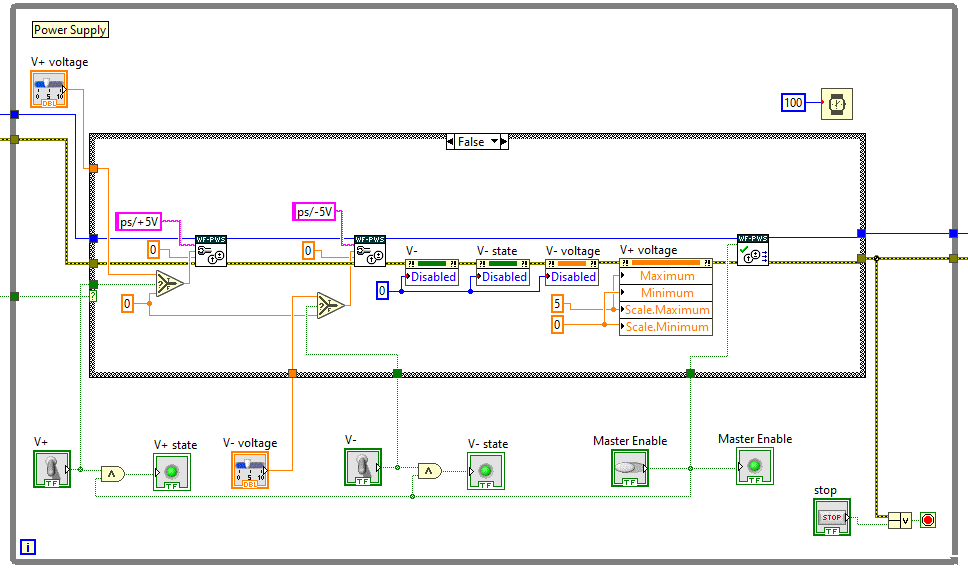
In this example the Block Diagram is separated in three parts with the help of decorative and functional structures. The first part named Device selection and initialization contains the combo box Device (control element), compares its output to predefined strings and initializes the Power Supplies instrument with the selected device name. This part has zero incoming and three outgoing signals: the Power Supplies instrument device handler, the errors and a flag which is true if the Digital Discovery, the ADP3450, or the ADP3250 was selected and false otherwise.

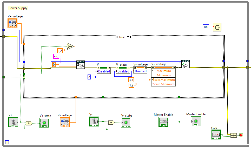
The next section is in a while loop, so it is repeated until a certain condition is met, with 100ms wait time between iterations. This part has as incoming signals the three from the previous section. The error signal and the device handler are cascaded to the Power Supply instrument settings, which also receive data from other control elements: voltage level sliders (V+ voltage and V- voltage) and power supply state switches (V+ and V-). These settings blocks are followed by property nodes, which are able to modify different parameters of existing blocks, in this case according to the device type, the V- channel is enabled/disabled and the V+ voltage slider’s range is modified. The next block turns the instrument on/off according to the state of the Master Enable switch. All these settings are inside a switch case, which changes constant parameters according to the selected device name (limits the voltage range for Digital Discovery). The loop is exited if there is an error, or the Stop button is pressed on the Front Panel.

If the loop is exited, the device handler and the errors are passed to the next section, which turns off the supplies, closes the instrument and sets all switches and virtual LEDs to off state, then displays an error message if there was one.

---

To run the VI, first on the front panel select the Test and Measurement device used, then press the Run button.

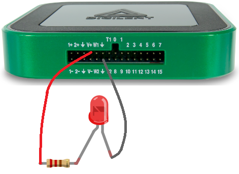
From here the power supply channels can be enabled with the help of the switches and adjusted with the help of the sliders. To visualize the output voltage, an LED should be connected in series with a 220Ω resistor between the V+ and the GND (down arrow) pins of the Test and Measurement device like in the image shown to the right. The program can be stopped with the Stop button on the Front Panel.

---

Digital I/O Example 1 - Virtual I/O

Download and unzip the provided example file digital_io_v2.zip then double click on it to open it with LabVIEW. All the instruments used in the example can be used in your own VI, play around and see what else you can create.

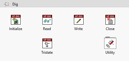
To access the digital I/O pins of the Test and Measurement device within LabVIEW, the following subvis are available in the Measurement I/O → Digilent WF VIs → Dig container:

• Initialize : allows the user to select the Digilent Test and Measurement device and sends the device handler to the other digital I/O subvis.
• Read: is used to read the state of a given set of digital I/O lines.
• Write: is used to set the state of a given set of digital I/O lines.
• Close: Closes the instrument when the program is terminated, making it available for other software (no instrument can be controlled by two programs at the same time).
• Other subvis for adding tristate buffers to the I/O lines, resetting the instrument or getting information about the state of the lines (tristated/static) are also available (these are not used in the example program).

---

A LabVIEW Virtual Instrument consists of two parts: the Front Panel and the Block Diagram. The Front Panel contains all controls and indicators for data in- and output and serves as a user interface when the program is running. The Block Diagram contains the blocks which are present on the Front Panel, but also other block which are necessary for information processing and the connections between these blocks. One can add a new block to both windows by right clicking on a blank space in the corresponding window and selecting the required block from a library. Blocks already present in the window can be modified by right clicking on the respective block. In the following paragraphs, this example's Front Panel and Block Diagram will be presented.

---

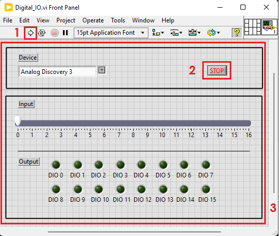
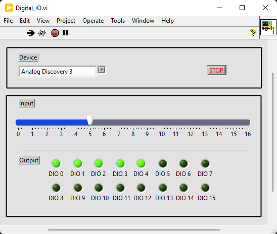
The Front Panel contains, along with the menu bar, the alignment setting, search buttons, etc. (see more at: LabVIEW Community Getting Started), the Run button (1) and the panel itself (3). Control and indicator objects are placed in the panel.

In this example the panel is separated in two parts with decorative elements. In the upper part there is a drop-down list with the name Device which is used to select the Test and Measurement device used. The Stop button (2) is also found here. With this button the program can be stopped, and the digital I/O lines all set to LOW.

The lower part contains a slider ranging from 0 to 16 (control) and 16 virtual LEDs, each one named after a digital I/O line. When the program is running, the slider determines how many of the digital lines will be HIGH. By moving the slider, the number of lines set to HIGH can be modified. The virtual LEDs indicate if a line is HIGH (they are lit if HIGH and dark if LOW).

---

The Block Diagram contains, along with the menu bar, the alignment setting, search buttons, etc. (see more at: LabVIEW Community Getting Started), the Run button (the program can also be started from here) and the panel itself. Control, indicator and data processing blocks and structures are placed in the panel and connected.

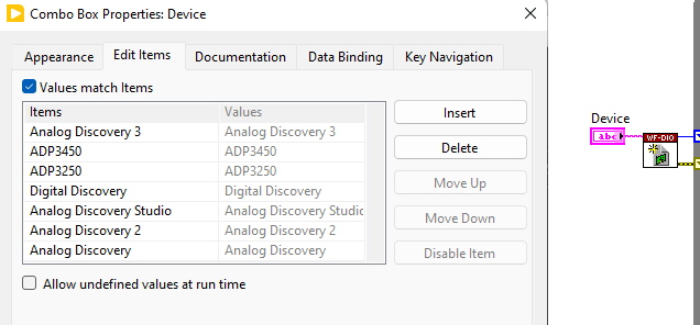
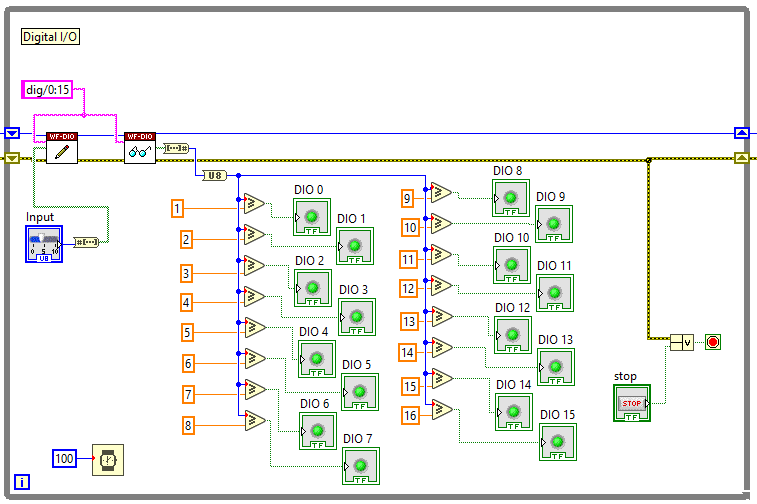
In this example the Block Diagram is separated in three parts with the help of decorative and functional structures. The first part named Device selection and initialization contains the combo box Device (control element) and initializes the Digital IO instrument with the selected device name. This part has zero incoming and two outgoing signals: the Digital IO instrument device handler and the error signal.

The next section is in a while loop, so it is repeated until a certain condition is met, with 100ms wait time between iterations. This part has as incoming signals the two from the previous section. The error signal and the device handler are connected to the DIO-Write block, which also receives data from the input slider. The number outputted by the slider is converted to a Boolean array with 8 elements, then the content of this array is written to the digital I/O lines. The error and instrument handle signals are connected then to the DIO-Read block. With the help of this block, the program reads the values of digital I/O lines 0 to 15, then converts the Boolean array to a number. This number is compared to constant values and the result of each comparison decides the state of the virtual LEDs. The loop is exited if there is an error, or the Stop button is pressed on the Front Panel. The instrument handle and the errors are sent towards the next part.

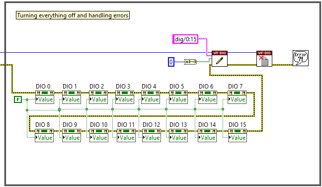
If the loop is exited, the state of all virtual LEDs is set to false (LEDs are turned off) with the help of property nodes, then an all 0 boolean array is written to the digital I/O lines (all lines are set to LOW). The instrument is closed making it available to other programs, then an error message is displayed, if there were any errors.

---

To run the VI, first on the front panel select the Test and Measurement device used, then press the Run button.

From here the state of digital I/O lines 0 to 15 can be set by the slider. The state of the pins is also read back and displayed with the help of the virtual LEDs . The program can be terminated with the Stop button on the Front Panel.

---

Digital I/O Example 2 - Simple Loopback

Download and unzip the provided example file digital_io_2_v2.zip then double click on it to open it with LabVIEW. All the instruments used in the example can be used in your own VI, play around and see what else you can create.

To access the digital I/O pins of the Test and Measurement device within LabVIEW, the following subvis are available in the Measurement I/O → Digilent WF VIs → Dig container:

• Initialize : allows the user to select the Digilent Test and Measurement device and sends the device handler to the other digital I/O subvis.
• Read: is used to read the state of a given set of digital I/O lines.
• Write: is used to set the state of a given set of digital I/O lines.
• Close: Closes the instrument when the program is terminated, making it available for other software (no instrument can be controlled by two programs at the same time).
• Other subvis for adding tristate buffers to the I/O lines, resetting the instrument or getting information about the state of the lines (tristated/static) are also available (these are not used in the example program).

---

A LabVIEW Virtual Instrument consists of two parts: the Front Panel and the Block Diagram. The Front Panel contains all controls and indicators for data in- and output and serves as a user interface when the program is running. The Block Diagram contains the blocks which are present on the Front Panel, but also other block which are necessary for information processing and the connections between these blocks. One can add a new block to both windows by right clicking on a blank space in the corresponding window and selecting the required block from a library. Blocks already present in the window can be modified by right clicking on the respective block. In the following paragraphs, this example's Front Panel and Block Diagram will be presented.

---

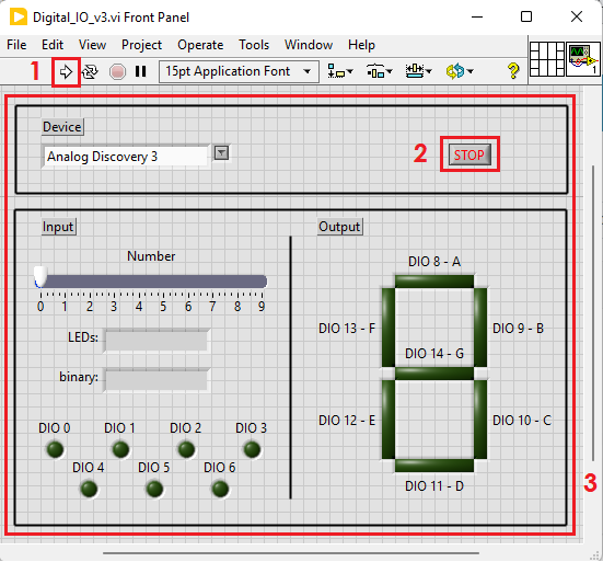
The Front Panel contains, along with the menu bar, the alignment setting, search buttons, etc. (see more at: LabVIEW Community Getting Started), the Run button (1) and the panel itself (3). Control and indicator objects are placed in the panel.

In this example the panel is separated in two parts with decorative elements. In the upper part there is a drop-down list with the name Device which is used to select the Test and Measurement device used. The Stop button (2) is also found here. With this button the program can be stopped, and the digital I/O lines all set to LOW.

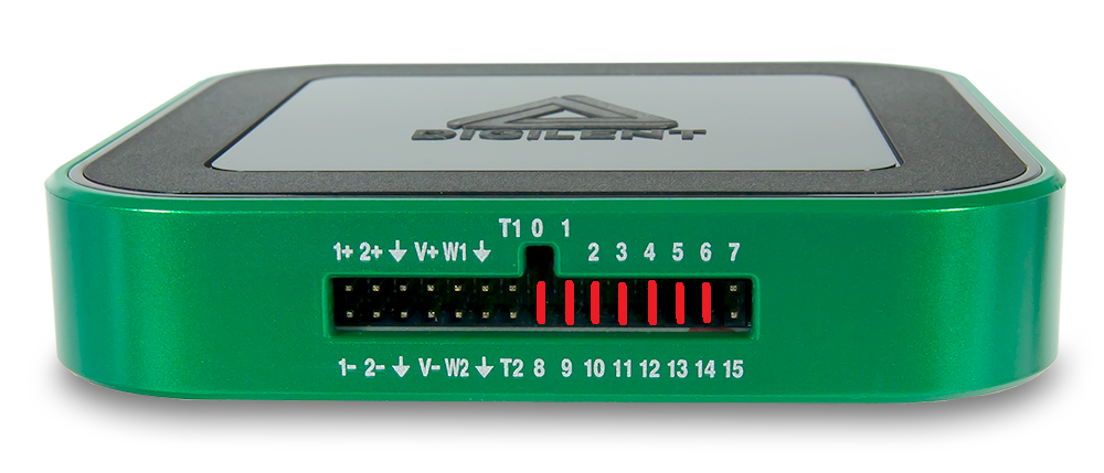
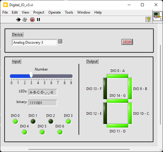
The lower part contains a slider ranging from 0 to 9 (control), two text fields (indicator), 7 virtual LEDs, and a seven-segment display. When the program is running, the number set with the slider is used to determine which segments should be lit on the seven-segment display, the list of these segments being displayed in one of the text fields. The other text field contains the binary number which should be written to the digital I/O lines 0-6. Virtual LEDs show the state of these lines. The seven-segment display is connected to digital I/O lines 8-14 and segments are turned on/off according to the state of these pins.

---

The Block Diagram contains, along with the menu bar, the alignment setting, search buttons, etc. (see more at: LabVIEW Community Getting Started), the Run button (the program can also be started from here) and the panel itself. Control, indicator and data processing blocks and structures are placed in the panel and connected.

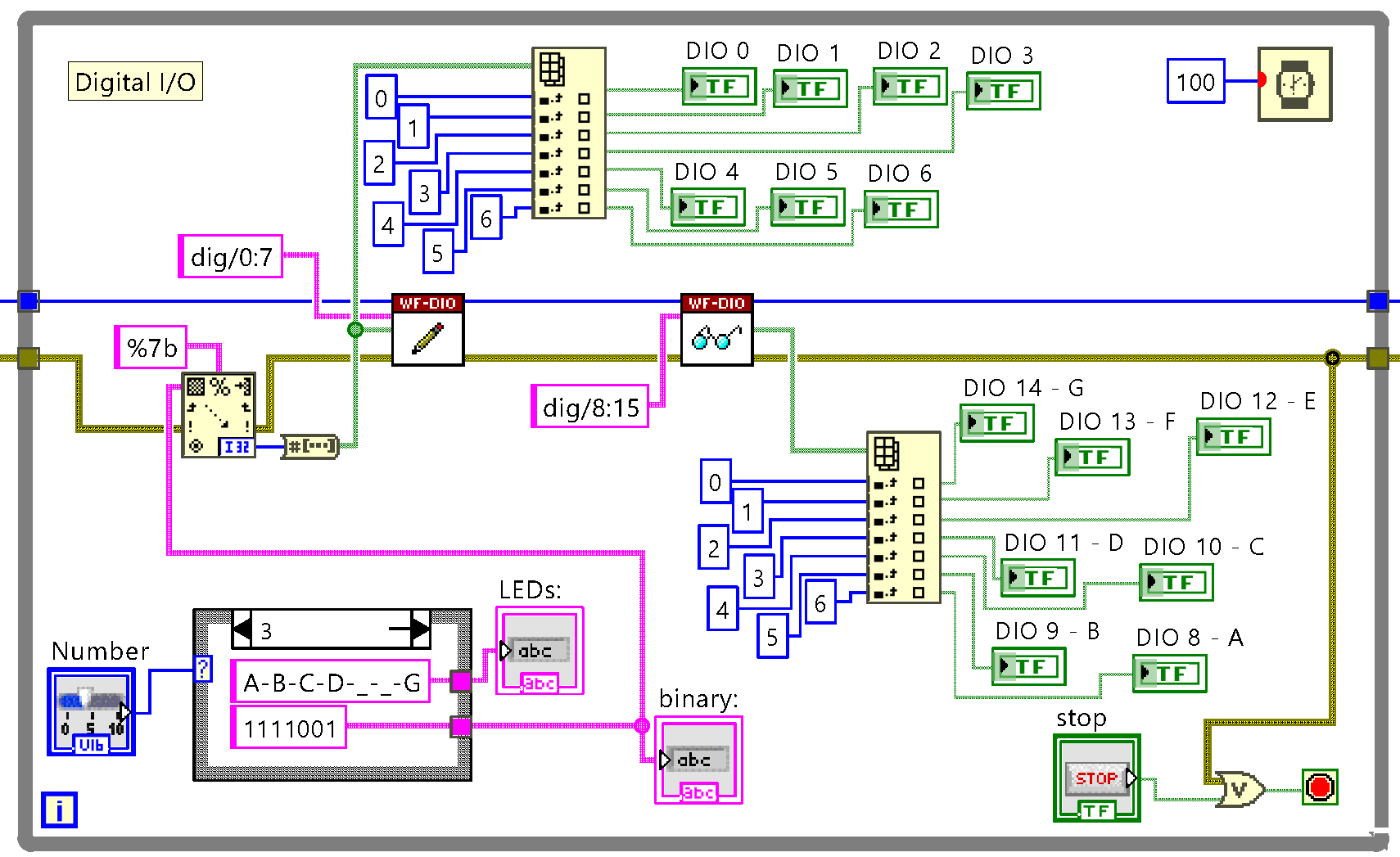
In this example the Block Diagram is separated in three parts with the help of decorative and functional structures. The first part named Device selection and initialization contains the combo box list Device (control element) and initializes the Digital IO instrument with the selected device name. This part has zero incoming and two outgoing signals: the Digital IO instrument device handler and the error signal.

The next section is in a while loop, so it is repeated until a certain condition is met, with 100ms wait time between iterations. This part has as incoming signals the two from the previous section. According to the number set on the slider, the two strings are determined, which will be displayed on the front panel. The binary string is then converted to a binary array and this array is sent to the digital I/O lines 0-6, as well as to the seven virtual LEDs showing the state of these lines.

As a next step, the state of the digital I/O lines 8-14 is read and the segments of the seven-segment display are controlled according to the received values. The loop is exited if there is an error, or the Stop button is pressed on the Front Panel. The instrument handle and the errors are sent towards the next part.

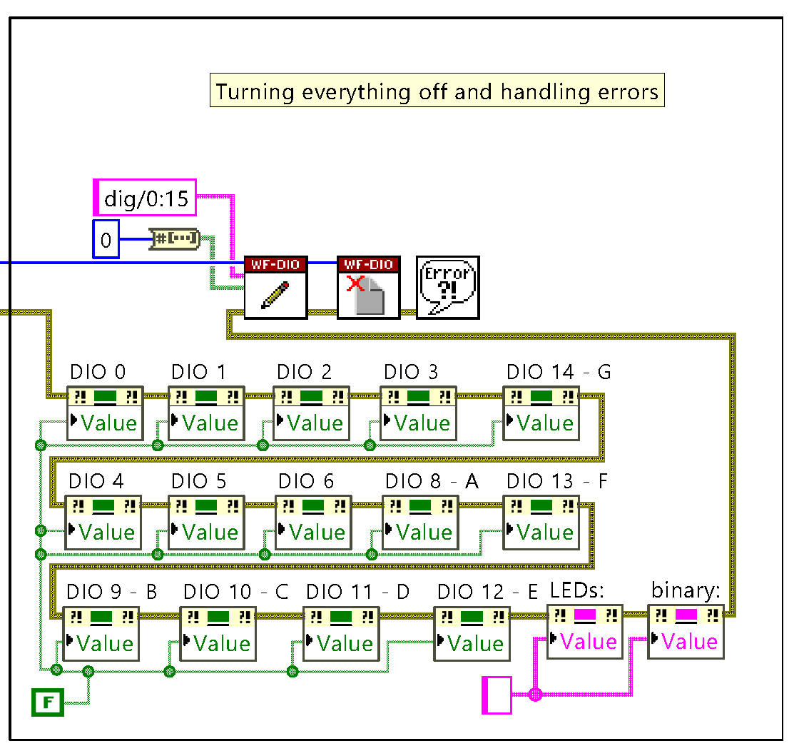
When the loop is exited, the state of all virtual LEDs is set to false (LEDs are turned off) with the help of property nodes, the strings are replaced with an empty string, then an all 0 Boolean array is written to the digital I/O lines (all lines are set to LOW). The instrument is closed making it available to other programs, then an error message is displayed, if there were any errors.

---

To run the VI, first on the front panel select the Test and Measurement device used, then press the Run button.

Connect DIO pins 0-6 to DIO pins 8-14, as seen in the diagram to the right. DIO lines 0-6 are used as output and are controlled by the slider. As the segments of the seven-segment display are connected to digital I/O lines 8-14, connecting the respective pins will display the number set on the slider. The program can be terminated with the Stop button on the Front Panel

---

Analog I/O Example

Download and unzip the provided example file frequency_sweep_v2.zip then double click on it to open it with LabVIEW. All the instruments used in the example can be used in your own VI, play around and see what else you can create.

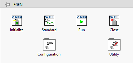
To use the Waveform Generator instrument within LabVIEW, the following subvis are available in the Measurement I/O → Digilent WF VIs → FGEN container:

• Initialize: allows the user to select the Digilent Test and Measurement device and sends the device handler to the other wavegen subvis.
• Standard: is used to set the function to be generated as well as the function’s amplitude, DC offset, duty cycle and frequency.
• Run: is used to start the function generator.
• Stop: stops the function generator.
• Close: Closes the instrument when the program is terminated, making it available for other software (no instrument can be controlled by two programs at the same time).
• Other subvis for generating arbitrary waveforms, returning data about the state of the function generator, resetting the instrument, etc. are also available (these are not used in the example program).

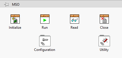
To use the Oscilloscope instrument within LabVIEW, the following subvis are available in the Measurement I/O → Digilent WF VIs → MSO container:

• Initialize: allows the user to select the Digilent Test and Measurement device and sends the device handler to the other scope subvis.
• Read: is used to aquire data from the sellected scope channel.
• Run: is used to start the oscilloscope.
• Stop: stops the oscilloscope.
• Close: closes the instrument when the program is terminated, making it available for other software (no instrument can be controlled by two programs at the same time).
• Analog: allows the user to select a channel and set the coupling type and the probe attenuation (which can be useful when using BNC probes).
• Analog Edge: is used to set the trigger level, the trigger slope and the trigger hysteresis for the selected channel.
• Timing: is used to configure the basic timing settings (like acquisition time and sample rate) of the instrument
• Other subvis for setting channel and trigger properties, returning data about the state of the oscilloscope, resetting the instrument, etc. are also available (these are not used in the example program).

---

A LabVIEW Virtual Instrument consists of two parts: the Front Panel and the Block Diagram. The Front Panel contains all controls and indicators for data in- and output and serves as a user interface when the program is running. The Block Diagram contains the blocks which are present on the Front Panel, but also other block which are necessary for information processing and the connections between these blocks. One can add a new block to both windows by right clicking on a blank space in the corresponding window and selecting the required block from a library. Blocks already present in the window can be modified by right clicking on the respective block. In the following paragraphs, this example's Front Panel and Block Diagram will be presented.

---

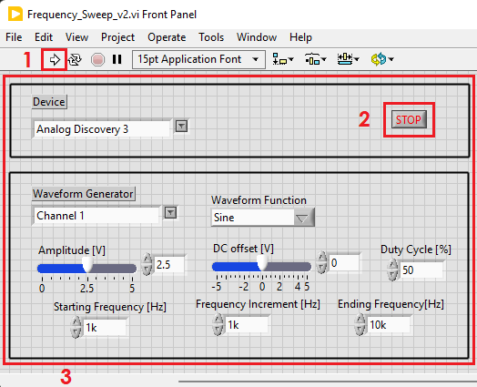
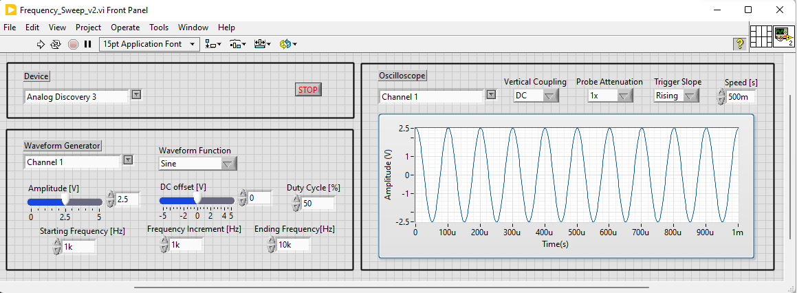
The Front Panel contains, along with the menu bar, the alignment setting, search buttons, etc. (see more at: LabVIEW Community Getting Started), the Run button (1) and the panel itself (3). Control and indicator objects are placed in the panel.

In this example the panel is separated in three parts with decorative elements. In the upper left part, there is a drop-down list with the name Device which is used to select the Test and Measurement device used. The Stop button (2) is also found here. With this button the program and both the Oscilloscope and Function Generator instruments can be stopped.

The lower left part contains all the control elements for the Wavegen instrument: channel and function selector drop-down lists, sliders and text boxes for setting the amplitude and DC offset voltages and text boxes for setting the duty cycle, the starting and ending frequency and the frequency increment of the sweep.

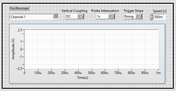
The right part named Oscilloscope contains four drop-down lists for scope channel selection, setting coupling type, setting trigger edge, and setting probe attenuation (by default this is set to 1X, should be modified if BNC probes are used) and a numeric control to set the speed of the measurements (it sets the acquisition time for every step). Beside of the control fields, a plot pane is also present: here will be displayed the measured signal. The range of the axis is set automatically.

---

The Block Diagram contains, along with the menu bar, the alignment setting, search buttons, etc. (see more at: LabVIEW Community Getting Started), the Run button (the program can also be started from here) and the panel itself. Control, indicator and data processing blocks and structures are placed in the panel and connected.

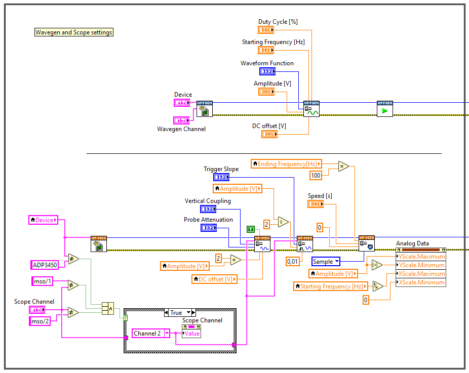
In this example the Block Diagram is separated in three parts with the help of decorative and functional structures. The first part is responsible for setting up the instruments according to the parameters retrieved from the Front Panel control elements. The setup processes of the Wavegen and the Scope instruments are done in parallel.

In the upper part, the selected channel of the Wavegen instrument is initialized, then the function to be generated and the function’s amplitude, duty cycle, and DC offset are set. The frequency of the generated signal is the starting frequency of the sweep. The Wavegen instrument is started with the Run block.

In the lower part, the Scope instrument is initialized, then the channel is selected. If the selected device is not the ADP3450, and Channel 3 or Channel 4 is the selected channel, the channel is set to Channel 2. The coupling and the probe attenuation are set. The vertical offset is equaled to the DC offset set at the Wavegen instrument and the vertical range is set to be two times the amplitude of the generated signal. Following this the trigger is attached to the selected Scope channel, the trigger slope is set according to the control element on the Front Panel, the trigger level is set to half of the amplitude of the generated signal and the trigger hysteresis is set to be 0.01V.

The acquisition time of the instrument is set accordingly to the Speed control element, the pretrigger time is set to 0 and the sampling frequency is set to 100 times the maximum signal frequency. The sampling frequency must be much higher then the maximum frequency of the sampled signal, because, if the signal is a rectangular or a triangular one, it contains high frequency harmonics as well at frequencies which are odd multiples of the fundamental frequency. To measure some of these components, according to the Nyquist criterion, $f_s$ (the sampling frequency) must be at least two times larger, than $f_m$ (the frequency of the measured component). With setting $f_s$ to $100f_{max}$ we can measure the first 25 harmonics of the signal, which gives a nearly perfect approximation.

The axis ranges of the plot pane are also set here: the X axis is ranging from 0 to the starting period and the Y axis is set to display the full peak-to-peak range of the signal.

The next part is in a while loop, so it is repeated until a certain condition is met, with 10ms wait time between iterations. This part has as incoming signals the instrument handles and error signals from the previous section, as well as the Wavegen instrument parameters (Duty Cycle, Starting Frequency, Waveform Function, Amplitude and DC offset) as local variables. The loop contains a Standard block (Wavegen settings), which receives as parameters the same ones as the Standard block in the previous section, but the Frequency is changed with every iteration, the new frequency being calculated as the sum of the starting frequency and the product between the frequency increment and the iteration index. If this calculated frequency becomes greater or equal to the ending frequency, the loop is exited. Other conditions which cause the program to exit the loop are errors appearing or if the Stop button is pressed on the Front Panel.

The loop also contains the Run block, which starts the Scope and takes a measurement, and a Read block connected to the indicator Analog Data, which is the plot pane on the Front Panel. The outgoing signals of this section are just the error signals and the instrument handles.

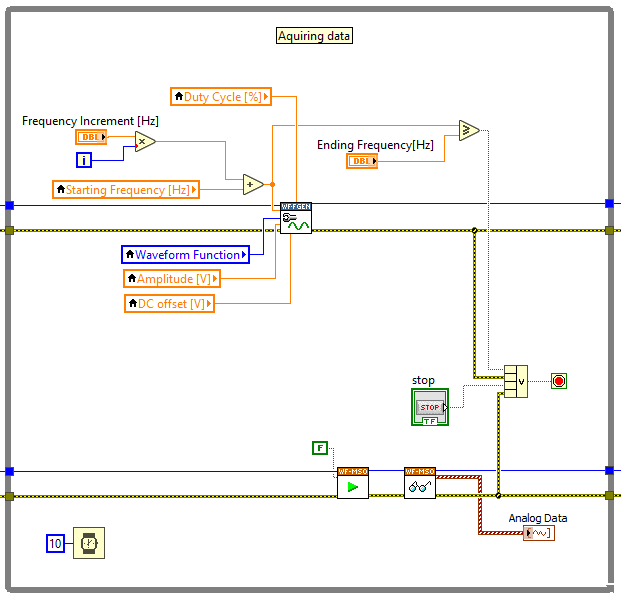
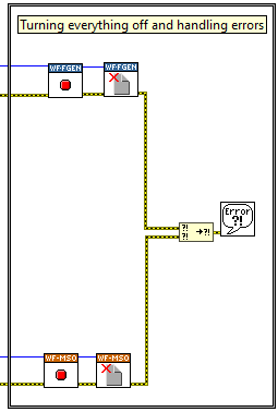
If the loop is exited, both instruments are stopped and closed, to make them available for other software. The two error signals are merged and handled: an error message is displayed, if there were any errors during execution.

---

To run the VI, first, on the Front Panel select the Test and Measurement device used, set the attributes of the desired waveform and the parameters of the frequency sweep, then press the Run button. The measurement can be stopped at any time with the Stop button, or is finished when the ending frequency is reached.

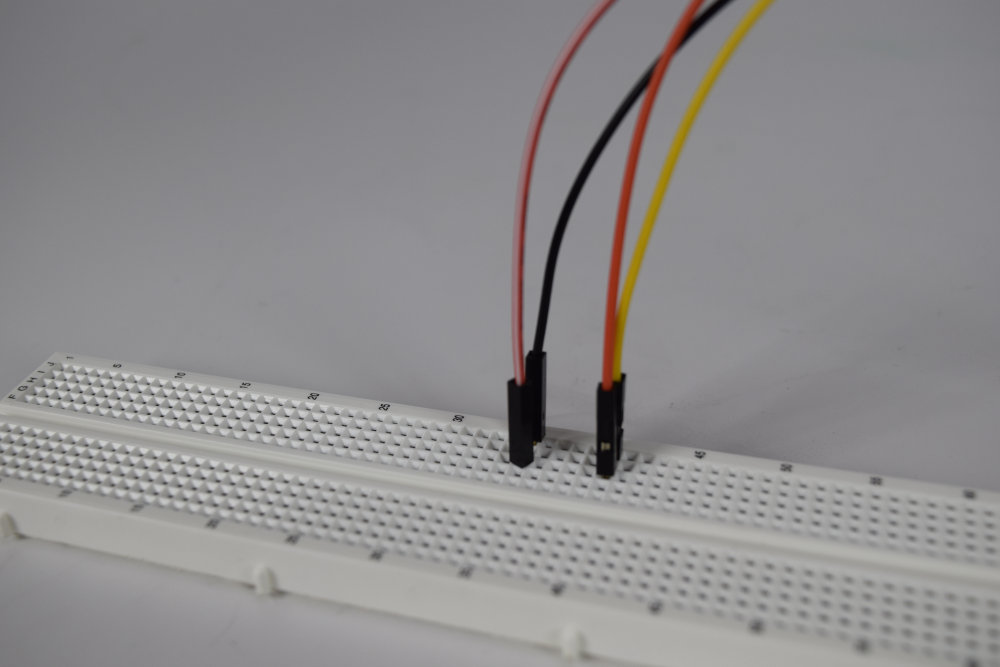
To to test the example , connect the Test and Measurement device's Oscilloscope Channel 1 pin (orange wire/circle) to the device's Wavegen Channel 1 output pin (yellow wire/circle). For devices that use differential input channels, such as the Analog Discovery 3 with MTE cables, make sure to connect the Oscilloscope Channel 1 negative pin (orange wire with white stripes) to the ground pin associated with Wavegen Channel 1 (black wire).

If your Digilent Test and Measurement device supports BNC cables, more options are available. Select your device, below, for instructions on using these cables.

Analog Discovery 3 with BNC Adapter

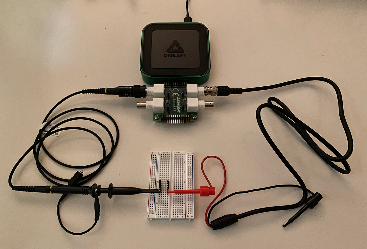
Connect the BNC Adapter to the Analog Discovery 3, as shown in the image to the right. Next, connect BNC cables to the Test and Measurement device's Oscilloscope Channel 1 BNC Connector and Wavegen Channel 1 BNC Connector. Connect the cables' probes to one another. Check the input probe's attenuation factor, as it will be used later to set up the software.

Note: For this demo, both ground wires were not connected together, because the Oscilloscope channel shares the same ground as the Wavegen channel. While BNC Probes are single-ended (as is the Waveform Generator hardware), a connected circuit must still share a common ground with the device. No more than one ground should be connected, in order to avoid the creation of ground loops, which may damage your device.

Note: When using BNC Probes, make sure to take note of the probes' bandwidth. When probes are used with an oscilloscope, the achievable bandwidth is limited by both the probes and by the scope. For example, using 1 MHz probes will limit the bandwidth to 1 MHz, even if that is below the Test and Measurement device's specified maximum.

Take note of the jumper that selects between AC and DC coupling on the BNC adapter. Either will work to measure the sine wave produced here, but some waveforms may find one setting or the other significantly more useful.

Analog Discovery Pro (ADP3450/ADP3250)

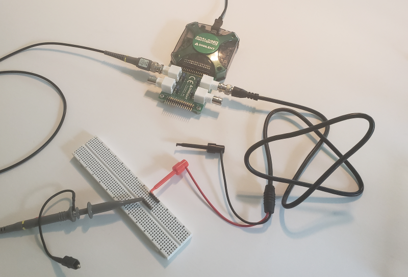
Connect a BNC oscilloscope probe to the Analog Discovery Pro's Oscilloscope Channel 1 connector and a set of BNC minigrabbers to its Wavegen Out Channel 1 connector. Connect these together, as pictured, to form a loopback circuit. Check the input probe's attenuation factor, as it will be used later to set up the software.

Note: For this demo, both ground wires were not connected together, because the Oscilloscope channel shares the same ground as the Wavegen channel. While BNC Probes are single-ended (as is the Waveform Generator hardware), a connected circuit must still share a common ground with the device. No more than one ground should be connected, in order to avoid the creation of ground loops, which may damage your device.

Note: When using BNC Probes, make sure to take note of the probes' bandwidth. When probes are used with an oscilloscope, the achievable bandwidth is limited by both the probes and by the scope. For example, using 1 MHz probes will limit the bandwidth to 1 MHz, even if that is below the Test and Measurement device's specified maximum.

Analog Discovery Studio

Connect BNC cables to the Test and Measurement device's Oscilloscope Channel 1 BNC Connector and Wavegen Channel 1 BNC Connector. Connect the cables' probes to one another. Check the input probe's attenuation factor.

Note: For this demo, both ground wires were not connected together, because the Oscilloscope channel shares the same ground as the Wavegen channel. While BNC Probes are single-ended (as is the Waveform Generator hardware), a connected circuit must still share a common ground with the device. No more than one ground should be connected, in order to avoid the creation of ground loops, which may damage your device.

Note: When using BNC Cables, make sure to take note of the probes' bandwidth. When probes are used with an oscilloscope, the achievable bandwidth is limited by both the probes and by the scope. For example, using 1 MHz probes will limit the bandwidth to 1 MHz, even if that is below the Test and Measurement device's specified maximum.

Note: The Analog Discovery Studio's BNC connectors are DC coupled.

Make sure to flip the switch that selects between BNC and MTE input for Oscilloscope Channel 1 towards the BNC connector.

Analog Discovery 2 with BNC Adapter

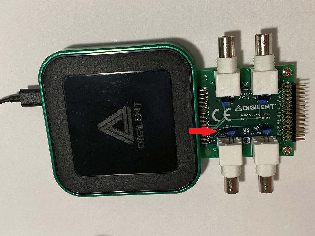
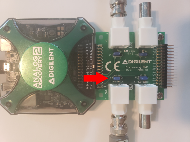
Connect the BNC Adapter to the Analog Discovery 2, as shown in the image to the right. Next, connect BNC cables to the Test and Measurement device's Oscilloscope Channel 1 BNC Connector and Wavegen Channel 1 BNC Connector. Connect the cables' probes to one another. Check the input probe's attenuation factor, as it will be used later to set up the software.

Note: For this demo, both ground wires were not connected together, because the Oscilloscope channel shares the same ground as the Wavegen channel. While BNC Probes are single-ended (as is the Waveform Generator hardware), a connected circuit must still share a common ground with the device. No more than one ground should be connected, in order to avoid the creation of ground loops, which may damage your device.

Note: When using BNC Probes, make sure to take note of the probes' bandwidth. When probes are used with an oscilloscope, the achievable bandwidth is limited by both the probes and by the scope. For example, using 1 MHz probes will limit the bandwidth to 1 MHz, even if that is below the Test and Measurement device's specified maximum.

Take note of the jumper that selects between AC and DC coupling on the BNC adapter. Either will work to measure the sine wave produced here, but some waveforms may find one setting or the other significantly more useful.

For more guides on how to use the Digilent Test and Measurement Device, return to the device's Resource Center, linked from the Test and Measurement page of this wiki.

For technical support, please visit the Test and Measurement section of the Digilent Forums.