Table of Contents
WaveForms Reference Manual
WaveForms is the virtual instrument suite for Digilent Test and Measurement devices.

The most up to date version of the following material is located in the Help tab in the WaveForms application. The Help tab is located to the right of the Welcome (Instrument menu) tab.

Features
- Cross platform
- In app scripting using JavaScript
Oscilloscope
- Triggers
- Edge, pulse, transition, hysteresis, hold-off
- XY, data, histogram, measurements view, cursor, hottrack
- Custom script measurements
- Stream acquisition
- Mixed mode with logic analyzer
- Data logging
- Standard and custom math, reference channels
- Reference data import from file and use in math channel
Waveform Generator
- Function, custom and sweep generator, AM/FM options, play mode
Voltage Supply
Data Logger
Logic Analyzer
- Simple (edge/level) trigger
- Signal, bus, SPI, I2C, UART protocol interpreters
- CAN, I2S, Custom protocol interpreters
- Data logging
- Stream acquisition
- Better cursors hottrack
Pattern Generator
- Clock, pulse, binary, Gray, Johnson counters…, custom
Static I/O
Network Analyzer
- Nyquist, Nichols, time view
- Reference Channels
- Attenuation setting
- Auto Range/Offset
- Magnitude units
Spectrum Analyzer
- Measurements, time view
- Components list
1. Getting Started with WaveForms
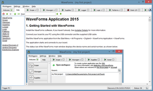
Install the WaveForms software, if you haven't already. Installer Details for more information.
Connect your board to your PC using the USB connector and the supplied USB cable.
Start the WaveForms application from the Start Menu > All Programs > Digilent > WaveForms > WaveForms.
The application starts and connects to your board.
The status bar of the WaveForms main window displays the device name and serial number, as shown below.
1.1. Troubleshoot WaveForms
Only one application can be connected to one board at a time. If you get the message “The selected device is being used by another application” check the taskbar for other applications in use.
If the application is not working as expected, try starting the WaveForms application from the MS Windows Start Menu > All Programs > Digilent > WaveForms > WaveForms Safe Mode or the WaveForms application with “clear” parameter.
See the device-specific troubleshooting:
1.2. Select an Instrument
The WaveForm's main window Welcome tab (shown above) has buttons for each instrument: Scope (Oscilloscope), Wavegen (Arbitrary Waveform Generator), Supplies (Supplies and Reference Voltages), Meters (Voltmeters), Analyzer (Logic Analyzer), Patterns (Digital Pattern Generator), Static I/O (Static Digital Input/Output), Bode (Network Analyzer), Spectrum Analyzer and Script instruments. The instruments can also be opened from the Welcome tab “+” (add) menu.
An instrument's button is disabled when the selected device or configuration does not support it.
The Settings menu contains the Options, the Device Manager, and Trigger PC.
The Workspace's Open, Save, and Save as buttons allow the user to load or save WaveForms workspaces.
When an instrument is closed, its state is saved and loaded when reopened. The New button creates a new workspace, which can be used to close the instruments that are currently open while also forgetting the last instrument configurations.
1.3. The Workspace and Project
The workspace refers to any open instruments and their current state. The workspace can be loaded and saved with the Open and Save/Save as buttons in the WaveForm's Welcome tab.
The workspace can be saved in one of the following modes selected by the save filter:
- All data: saves all data; buffered Oscilloscope and Logic Analyzer acquisitions, Oscilloscope reference channel samples, custom AWG waveforms, and Pattern Generator custom data are saved. This option can result in a file size of several megabytes.
- Reduced size: saves only the Oscilloscope reference channels and selected buffer, selected Logic Analyzer buffer, selected custom AWG waveforms, and Pattern Generator custom data.
The workspace files are associated with WaveForms. When you open a workspace (double-click on a *.dwf3work file) and WaveForms is running, it will be opened with the last used application instance. Otherwise, if WaveForms is not currently running, it will open with a new application instance.
The project refers to an instrument and its current state. The project can be loaded and saved with the Open and Save buttons in each instrument.
The project files are associated with WaveForms. When you open a project (double-click on a *.dwf3scope, *.dwf3wavegen, *dwf3analyzer, … file) and WaveForms is running, it will be opened with the last used application instance. Otherwise, if WaveForms is not currently running, it will open with a new application instance.
2. Options
The Options window allows you to select various display and configuration preferences.
To open the Options window, select the Settings / Options menu from the WaveForms window.

- Instrument windows: Specifies how the instrument windows are opened; it can be one of the following options:
- Separate: separate windows.
- Tabs: tabs in main window.
- MDI: multiple document interface.
- Style: Select the application GUI style. The available options depend on the system. It is recommended to restart the application after a change.
- Analog/Digital color: Selects the color for analog or digital instrument plots.
- Graphics optimization: adjusts the balance between quality and speed.The following options depend on the selected device.
- Trigger #: Trigger pin can be configured to be input (default) or be driven by an instrument's trigger signal.
3. Device Manager
The Device Manager allows you to select the device and configuration to use with the WaveForms application.
To open the Device Manager, select the Settings / Device Manager menu or click on the window's status bar device button from the WaveForms window.

Devices list: Select the device you want to use. The Demo device allows you to explore WaveForms's capabilities without a physical device being connected to the PC.
Configurations: Select the configuration you want to use for the selected device. The configurations have different device buffer-memory distributions for the instruments and other capabilities, like number of pins or channels.
Calibrate list: The Calibrate button opens the Calibration window.
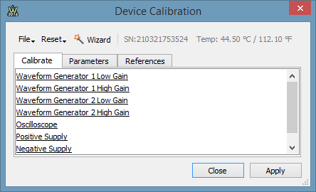
4. Device Calibration
The Device Calibration window allows you to calibrate (fine-tune) a device's analog components, like the read-voltage levels of the Oscilloscope or Voltmeters, the output level of the Waveform Generator or Adjustable Power Supplies of the Electronics Explorer board, or the Oscilloscope and Waveform Generator of the Analog Discovery device.
Start the Device Calibration window from the WaveForms main window Settings / Device Manager.
The following window will open. The items in the calibration list depend on the selected device type.
- File:
- Open: loads a previously saved calibration parameter file.
- Save: stores the current calibration parameters to a file.
- Reset:
- Discard changes: cancels any changes made after opening the Device Calibration window or pressing the Apply button.
- Load Factory: loads the default calibration parameters.
- Reset to Zero: resets the calibration parameters to zero.
- Apply: saves the calibration changes made to the device.
- Calibration tab: allows you to double-click a listed item to start its calibration.
- Parameters tab: allows you to review the calibration parameters.
- References tab: allows you to review the measured calibration and reference values.
5. Common Interfaces
5.1. Menu
The menu strips of the instrument windows generally have:
- File menu where project open and save operations can be performed.

- New
- Empty: opens a new empty instrument.
- Clone: opens a new instrument with the same configuration as the one of the current instrument.
- Open Project: opens an instrument project.
- Save Project: saves an instrument project to file.
- Export: exports data or screenshot from one of the opened views. See Export for more information.
- Close: closes the instrument.
- Control menu with single, run, and stop controls.

- Single: starts a single acquisition.
- Run: starts repeated acquisitions or continuous generation.
- Stop: stops the instrument.
- View menu where child windows, toolbars, and other visual options can be selected.
- Window menu contains links to the main window and all open instrument windows of this application.

- Help menu contains:
- Browse: opens Help in the default browser.
- Home Page: opens the Digilent web page.
- About: opens the About dialog to show the software version and support contact.
5.2. Lists
The mouse operations for lists are as follows:
- left mouse click: selects an element.


- shift and left mouse click: selects an element range.


- control and left mouse click: adds an element to the selection list.

- mouse move with pressed left button on row header: moves the selected elements.

- Delete button: removes selected elements.
 Select

 Select

Move

5.3. Plots
The center of the plot is marked with grid lines. Each vertical and horizontal line constitutes a major division. For linear scales these are laid out in a 10-by-10 division pattern. The tick marks on the sides between major divisions are called minor divisions. For logarithmic scales major tick ticks are show for each decay value and minor ticks for 2,3,4… points.
The plot sides allow scaling adjustment with left-button mouse drag the offset/position is changed and with right-button or mouse wheel or left-button and Alt key pressed the range is changed. The Ctrl key speeds up and Shift slows down the respective operation.
Each plot has a drop-down button in the top-right corner or mouse right-click shows menu containing options for:
- Color: selects the color theme for this plot.
- Plot Width: sets the thickness of the waveform, expressed as points.
The HotTrack lets you take measurements by moving the mouse cursor. This shows a vertical cursor and the values at intersections with waveforms. This can be enabled and disabled with the toggle button in the top-right corner or mouse double click on the plot. Click on the plot locks or unlocks the hottrack to current position.
The Cursors are used to measure the amplitude, to indicate certain places on the waveform, such as band or channel limits. Using delta cursors, you can make measurements that deal with power change with frequency or time. These can be added by pressing the X button in the plot bottom left corner. The Y cursors in Scope main time plot can be added by Y button in top right corner. The first cursors is by default added as normal cursor, the following ones as delta of this, showing the difference. The cursors position can be modified by mouse drag, keyboard arrow keys or adjustment control in cursor's drop-down menu. Mouse button middle click removes the cursor. The cursors can be selected with the channel number shortcut, pressing 1, 2,..
The Cursor view enabled in the instrument's View menu shows the position and measurements in table. The cursor's drop down menu and the table as well, contains adjustment controls for the reference cursor selection, position, delta value relative to reference cursor and remove button. For horizontal cursors the position is expressed in horizontal axis unit and vertical value is shown in intersection with each waveform.
5.4. Docking Windows
The docking windows functionality gives you flexible organization of docking windows within the parent window.

The windows can be dragged by their top border. When dragging is above the margins of the parent window, it will indicate the drop region. If you release the mouse, the child window will be docked to the corresponding margin. If you position a child window above another child window with same parent, it can dock in tabular mode. Releasing a window outside of drop regions makes the window float.
5.5. Export
The Export dialog lets you save the data or screenshot. The data can be saved as CSV (comma separated values) or TXT (tab delimited values). By checking the save options, the following information will also be saved:
- Comments: title, device name, serial number, and software version.
- Header: column header names, for instance: Time (s), C1 (V), etc.
- Label: first column, depending on the selected source this can be time or frequency.
The screenshot image can be saved in various image formats.

5.6. Script
The script editor uses java-script language to create custom Math channel in Scope, custom waveform pattern in WaveGen and Meter channel function. These expect mathematical function which will be called for each sample to transform input value (data or X).
The specific objects and variables available in each of these can be found under the Insert menu Locals group. Beside these the standard script elements are the following:
- mathematical operations: addition “+”, subtraction “-”, multiplication “*”, division “/”, reminder “%”.
- brackets: parenthesis (), square brackets []
- constants: Math.E, Math.PI, Math.LN2, Math.LN10
- functions: Math.log (logarithm), Math.pow (power), Math.min (minimum), Math.max (maximum), Math.sqrt (square root), Math.sine, Math.cos, Math.tan, Math.acos, Math.atan, Math.atan2, Math.abs (absolute value), Math.round, Math.floor, Math.ceil
The custom measurements in Scope expects a more complex script, where the value in the last line is the result. Here you probably need to implement loop to process the acquisition data.
For further information see Script Code.
5.7. Logging
The Logging tool allows you to save data on each acquisition or executing custom script code. This is available in Scope, and Analyzer instruments.


- Execute: selects when the logging will be executed.
- Manual: only by pressing the Save button.
- Each acquisition.
- Each triggered acquisition.
- Index: is the variable that is automatically incremented after each save operation and can be used in file naming in Simple mode.
- Maximum: specifies the limit for Index value for which Simple save operation is performed.
- Export
- Source: selects the source of saving which can be acquisition or an opened view. The following options are available:
- Comments: title, device name, serial number, date and time.
- Header: column header names, for instance: Time (s), C1 (V), etc.
- Label: first column, depending on selected source this can be time or frequency.
- Path: specifies the folder where the files will be saved.
- File: specifies the file name. See the options in the right of the File field for available regular expressions to generate file names. Number sign (#) will be replaced by Index and more “#” signs indicate zero padding the number. The expression between square brackets will be replaced by date and time:
| Expression | Output |
|---|---|
| d | the day as a number without a leading zero (1 to 31). |
| dd | the day as a number with a leading zero (01 to 31). |
| ddd | the abbreviated localized day name (e.g., 'Mon' to 'Sun'). Uses the system locale to localize the name. |
| dddd | the long localized day name (e.g., 'Monday' to 'Sunday'). Uses the system locale to localize the name. |
| M | the month as a number without a leading zero (1-12). |
| MM | the month as a number with a leading zero (01-12). |
| MMM | the abbreviated localized month name (e.g., 'Jan' to 'Dec'). Uses the system locale to localize the name. |
| MMMM | the long localized month name (e.g., 'January' to 'December'). Uses the system locale to localize the name. |
| yy | the year as a two digit number (00-99). |
| yyyy | the year as a four digit number. |
| h | the hour without a leading zero (0 to 23 or 1 to 12 if AM/PM display). |
| hh | the hour with a leading zero (00 to 23 or 01 to 12 if AM/PM display). |
| H | the hour without a leading zero (0 to 23, even with AM/PM display). |
| HH | the hour with a leading zero (00 to 23, even with AM/PM display). |
| m | the minute without a leading zero (0 to 59). |
| mm | the minute with a leading zero (00 to 59). |
| s | the second without a leading zero (0 to 59). |
| ss | the second with a leading zero (00 to 59). |
| z | the milliseconds without leading zeroes (0 to 999). |
| zzz | the milliseconds with leading zeroes (000 to 999). |
| AP or A | use AM/PM display. A/AP will be replaced by either “AM” or “PM”. |
| ap or a | use am/pm display. a/ap will be replaced by either “am” or “pm”. |
| t | the timezone (for example “CEST”). |
- Script allows you to perform custom save operations with the instrument object (Scope or Logic). See Script for more details.
6. States
The active instruments (Oscilloscope, Wavegen, Logic, and Patterns) step through states while acquiring or generating a signal.
From each of these instruments, multiple instances can be opened at a time; however, only one instance can be active. When more instruments of the same type are opened, the last used instance (after pressing Run or Stop) controls the device. The others display a Busy status.
6.1. Acquisition States
- Ready: instrument is not running.
- Config: instrument is under configuration or acquisition buffer is prefilled.
- Armed: instrument is armed and is waiting for a trigger event to occur.
- Trig'd: acquisition is triggered. It is useful when repeated acquisitions are running to see whether the trigger condition was met or the acquisition was automatic.
- Auto: acquisition is automatically started and not by the trigger condition.
- Done: single acquisition is completed.
- Stop: instrument was stopped.
- Scan: instrument is running in scan screen or shift mode.
- Error: is displayed if you have just disconnected the device from the PC.
6.2. Generator States
The following diagram illustrates the states of the Arbitrary Waveform Generator and Digital Pattern Generator.

- The instrument leaves the Ready state if it is started with the Run or Run All buttons or any changes have been made.
- The instrument is in the Config state for a short while when the new configuration is applied. It then goes to the Armed state if it is started or changes have been made while running. Otherwise, it goes back to the Ready state.
- In the Armed state, it waits for the trigger. The trigger can come from any other instrument or external source. If 'None' trigger source has been specified, signal generation starts immediately.
- It pauses in the Wait state until the specified wait time elapses.
- In the Run state, signal generation is enabled until the specified run-time elapses. If the continuous option has been specified, it stays in this state until stopped.
- The (Trigger)–Wait–Run cycle is repeated the number of times specified by the Repeat parameter, then it goes to the Done state. If the infinite option has been specified, it always goes back to the Wait state until it is stopped.
The Repeat cycle can be configured to include Trigger or not.
- Wait–Run mode: once triggered, will repeat the wait-run cycle for the specified times.
- Trigger–Wait–Run mode: waits for the trigger event each time before entering the Wait and Run states.
If any setting (frequency, duty, signal type, etc.) is modified, from any state, it goes right to the Config state. If the instrument was running, it will be started again.
7. Triggers
The trigger event is the rising edge of the trigger signal. The Electronics Explorer board has four trigger input pins. They are used by the Oscilloscope, Arbitrary Waveform Generators, Logic Analyzer, and Digital Pattern Generator instruments. The instruments output a trigger signal as long as they are in Run state.
Any of these instruments can be triggered by any of the trigger signals coming from external pins or the other instruments.
The Waveform Generator channels can function as independent instruments, having their own controller, or in synchronized mode when the selected channels are controlled by one state controller.
The input instruments (Oscilloscope and Logic) have a trigger detector based on their input channels.
The Trigger PC event is generated by pressing the button under the main window device menu. On the Electronics Explorer board, this trigger event is generated when the board switch is turned to the on position as well.
The None trigger mode configuration in the instruments means that acquisition or generation doesn't wait for a trigger, it starts immediately.
The Auto trigger mode for input instruments means that if the trigger condition doesn't appear in approximately two seconds, acquisition is started automatically.
In multiple acquisition mode, when the instruments switch to Auto trigger, subsequent acquisitions are made without waiting for timeout as long as a trigger event does not occur and the configuration is not changed. When a new trigger event occurs or the configuration is changed, the current acquisition is finished and the next one waits for the trigger. It is also the best mode to use if you are looking at many signals and do not want to set the trigger each time.

8. Installer
The Mac OS® X application is packaged in an Apple Disk Image file, like: digilent.waveforms_3.0.0.dmg. To install the application, copy it from the image to the Applications folder.
For Linux®, the application is available in DEB and RPM packages for 32 and 64-bit systems. The required Digilent Adept Runtime must be installed separately.
The installers for Microsoft Windows®, like digilent.waveforms_v3.0.0.exe, has the following command line arguments:
- /S (silent mode) installs or updates WaveForms without the installation wizard. If you use this option while WaveForms is running, installation might fail.
- /CurrentUser or /AllUsers creates and installs shortcuts for the current user or for all users. This option works for fresh installs of WaveForms. Updates or additions use the option from the first installation. To change this option, WaveForms must be uninstalled and then installed again.
- /Update only already installed components are selected.
The following are the command line arguments for the WaveForms application:
- -safe-mode: launches the application in safe mode without loading the saved options and recent workspace list.
- *.dwf3work: loads the workspace.
For projects, the instrument is opened and project loaded:
- *.dwf3scope: Scope - Oscilloscope.
- *.dwf3wavegen: Wavegen - Waveform Generator.
- *.dwf3logic: Logic Analyzer.
- *.dwf3patterns: Pattern Generator.
- *.dwf3supplies: Power Supplies.
- *.dwf3logger: Data Logger.
- *.dwf3static: Static I/O.
- *.dwf3network: Network Analyzer.
- *.dwf3spectrum: Spectrum Analyzer.
- *.dwf3script: Script.
In order for these options to work, the path where the application is installed has to be selected in the command line.
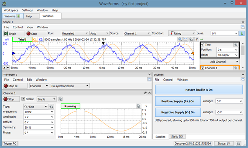
Oscilloscope
An oscilloscope (or “scope”) allows you to view signal voltages, typically in a two-dimensional graph where one or more electrical potential differences (on the vertical axis) are plotted as a function of time or of some other voltage (on the horizontal axis).
Most of the time, oscilloscopes are used to show events that repeat with either no change or change slowly.

1. Menu
See Menu in Common Interfaces.
1.1. View

- Add Zoom: adds a new Zoom view.
- Add XY: adds a new XY view.
- FFT: opens/closes the FFT view.
- Histogram: opens/closes the Histogram view.
- Persistence: opens/closes the Persistence view
- Data: opens/closes the Data view.
- Measure: opens/closes the Measurements.
- Logging: opens/closes Logging tool.
- Audio: opens/closes Logging tool.
- X Cursors: opens/closes X Cursors view.
- Y Cursors: opens/closes Y Cursors view.
- Digital: enables/disables the Digital Channels.
2. Control

The Control toolbar allows you to stabilize repeating waveforms and capture single-shot waveforms. By default, this only shows the important options. The down/up arrow in the top left corner shows/hides the other features.
- Single button: starts a single acquisition.
- Run/Stop button: starts a repeated, continuous, or stream acquisition (see Run mode). While the acquisition is in progress, the Run button becomes the Stop button.
- Run: The options in Run mode select the action of the Run button and are the following:
- Repeated: the Run button starts repeated acquisitions.
- Scan Screen: scan acquisition where the sampled data is drawn from left to right. When the right corner is reached, the signal curve plot continues from the left.
- Scan Shift: similar to the screen mode, but when the signal plot reaches the right corner, the curve plot slides to the left.
- Stream: allows capturing large number of samples at lower rates. In this mode, the samples are streamed through the USB limiting the rate (depending on the system and other connected devices) at about 1M samples/sec.
Selecting the scan modes (Screen and Shift) will change the time base to be at least 1 second span, 100 ms/division. Adjusting the time base to lower than this value will change to Repeated mode.
- Buffer: The performed acquisitions are stored in the PC buffer in time order. This makes it easy to review a series of repeated acquisitions. The new acquisitions are stored after the currently selected buffer position. If you change the position in the buffer and start a new acquisition, the positions after the selected one will be lost.
- Mode: The three trigger modes are:
- Normal: the acquisition is triggered only on the specified condition. The oscilloscope only sweeps if the input signal reaches the set trigger point.
- Auto: when the trigger condition does not appear in 2 seconds, the acquisition is started automatically. In repeated acquisition mode, when the instrument switches to auto trigger, the next acquisitions are made without waiting again to timeout while a trigger event does not occur and the configuration is not changed. When a new trigger event occurs, or the configuration is changed, the current acquisition will be finished and the next one will wait for the trigger again. It is also the best mode to use if you are looking at many signals and do not want to bother setting the trigger each time.
- None: the acquisition is started without a trigger.
- Auto Set button: performs automatic adjustment of the enabled real and mathematic channels, and trigger configuration according to the input signals. The offset and range of the real channels is determined by the minimum and maximum input levels of one second time span. The trigger is set to rising edge of the channel with the lowest frequency and higher amplitude input signal.
- Source: The trigger source selects the oscilloscope channel that is used for the trigger. Other instruments or external trigger signals can be used to trigger the oscilloscope.
- Type: The trigger type selects between edge, pulse, and transition.
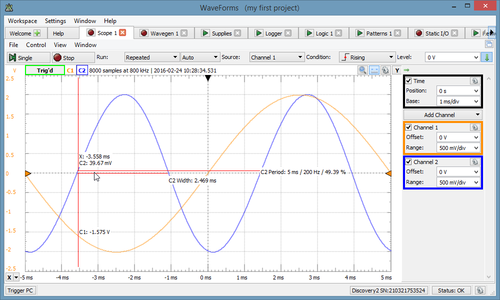
- Edge: Edge triggering is the basic and most common type. For edge triggering, the trigger level and slope controls provide the basic trigger point definition. The trigger circuit acts as a comparator. You select the slope and voltage level of one side of the comparator. When the trigger signal matches your settings, the oscilloscope generates a trigger.
The slope-condition control determines whether the trigger point is on the rising or the falling edge of a signal. A rising edge is a positive slope and a falling edge is a negative slope. The level control determines where the trigger point occurs on the edge. The following figure shows you how the trigger slope and level settings determine the waveform display.


- Pulse: If the trigger type is set to Pulse, then the oscilloscope will trigger if a positive/negative pulse has a larger/smaller length than the one already set by the user. For example, if the pulse is smaller than the length set, and the triggering condition is set to more, the oscilloscope will not trigger.
The picture below shows a positive pulse trigger configured for less than 200 µs.

The picture below shows a positive pulse trigger configured for time-out at 200 µs.

The picture below shows a positive pulse trigger configured for more than 200 µs.

- Transition: The transition trigger is similar to the pulse trigger, but here the transition time of a signal is compared with the specified length. The low and high transition levels are specified by the hysteresis window.
The picture below shows a rising transitions trigger from -3V to +3V configured for less than 200 µs.
![]()
The picture below shows a rising transitions trigger from -3V to +3V configured for time-out at 200 µs.
![]()
The picture below shows a rising transitions trigger from -3V to +3V configured for more than 200 µs.
![]()
- Condition: The trigger condition for Edge and Transition type selects between rising or falling edge. For Pulse trigger it selects between positive or negative pulse.
- Level: The trigger level is the adjustable voltage level at which the scope triggers when the trigger input crosses this value. See Hysteresis and Type.
- Hysteresis: Using hysteresis, low and high levels are determined (the trigger level plus and minus the hysteresis value). When the signal level exceeds the high level, it is considered as high and will stay high until falling below the low level. This is used to avoid bouncing caused by signal noise and also to specify the transition trigger conditions. The Auto option uses 1% of the specified trigger channel range value.

The picture below shows how, without hysteresis, the trigger event also occurs on the falling edge of the input signal due to signal noise.

- Length Condition: The trigger length condition selects between less, time out, or more for pulse length or transition time. See Pulse and Transition trigger.
- Trigger Length: The trigger length specifies the minimal or maximal pulse length or transition time. See Pulse and Transition trigger.
- Holdoff: The trigger holdoff is an adjustable period of time during which the oscilloscope will not trigger. This feature is useful when you are triggering on complex waveform shapes, so the oscilloscope triggers only on the first eligible trigger point.
The following figure shows how the trigger holdoff helps to create a usable display.
 Trigger with 10ms holdoff.
 '
Trigger without holdoff.
'
Trigger without holdoff.
The holdoff length should be around the maximum burst length, preferably a little bit more, but not less than this. For the above situation the holdoff value should be around 6ms, but lengths between 6 and 15 ms are also acceptable.
- Gear:
- Buffers: Specifies the number of buffers.
- Filter: The trigger sample selects the sample mode that will be used by the trigger detector. This can be different from the one used for acquisition, which is why the trigger event might not be visible on the acquired data. The Auto option uses a filter based on the selected trigger source channel Sample Mode.
3. Channels
This toolbar contains the time and channel configuration groups. The toggle button in the top-left corner enables/disables the auto hiding of this toolbar.

The Add Channel button opens a drop-down with the following options:
- Math: creates a new simple or custom math channel.
- Reference: the selected channel waveform is saved as a reference channel or waveform data imported from file.
- Digital: creates a new digital channel and enables the digital channels.
The check-box before the group name enables or disables the respective channel. The drop-down properties button in the top-right corner allows you to configure the channel properties. The math and reference channels also have a close button.
3.1. Time Group


Use the time group to position and scale the waveform horizontally using the time base and the horizontal trigger position controls.
- Position: The horizontal position control moves the waveform left or right to exactly where you want it on the screen. It actually represents the horizontal position of the trigger in the waveform recording. Varying the horizontal trigger position allows you to capture what a signal did before a trigger event (so-called “pre-trigger viewing”).
Digital oscilloscopes can provide pre-trigger viewing because they constantly process the input signal, whether a trigger has been received or not. Pre-trigger viewing is a valuable troubleshooting aid. For example, if a problem occurs intermittently you can trigger on the problem, record the events that led up to it, and possibly find the cause.
- Base: The time base (seconds/division) setting from the channel configuration toolbar lets you select the rate at which the waveform is drawn across the screen. This setting is a scale factor. For example, if the setting is 1 ms, each horizontal division represents 1 ms and the total screen width represents 10 ms (ten divisions). Changing the sec/div setting allows you to visualize longer or shorter time intervals of the input signal.
In the property drop-down, the following can be configured:
- Position as division: selects the unit of the position parameter, division, or seconds.
- Range Mode: selects the display mode for time base (per division, plus-minus, and full).
- Rate: adjusts the sample rate.
- Samples: adjust the number of samples to acquire.
Digital:
- Rate: adjusts the sample rate for digital channels.
- Samples: adjust the number of samples to acquire for digital channels.
- Noise: selects to acquire digital noise samples in half of the digital buffer.
- Update: this specifies the time period at which the application will check the oscilloscope device status and read the acquired data in repeated Run mode. Increase the time to reduce the update rate.
3.2. Real Channels


Use the real channel (vertical controls) to position and scale the waveforms vertically using the offset and range controls for each channel.
- Offset: The offset (vertical position) control lets you move the waveform up or down to exactly where you want it on the screen. The offset is the voltage difference between the center line of the oscilloscope screen and the actual ground. This difference is generated by an internal offset voltage source.
- Range: The range (volts/division) controls determine the vertical scale of the graph drawn on the oscilloscope screen. The volts/div setting is a scale factor. For example, if the volts/div setting is 2 volts, then each of the ten vertical divisions represents 2 volts and the entire screen can show 20 volts from bottom to top. If the setting is 0.5 volts/div, the screen can display 5 volts from bottom to top, and so on. The maximum voltage you can display on the screen is the volts/div setting multiplied by the number of vertical divisions.
In the property drop-down, the following can be configured:
- Color: sets the channel waveform color.
- Offset as division: selects the unit of the offset parameter, division, or voltage.
- Noise: shows or hides the noise band (min/max values).
- Range mode: selects the display mode for the range of the channels (per division, plus-minus, and full).
- Attenuation: specifies the used probe attenuation.
- Sample Mode: sets the acquisition sample mode. The oscilloscope AD converter works at a fixed frequency. Depending on the time base setting and the size of the oscilloscope buffer, the sampling frequency can be less than the AD conversion frequency. For instance, if the AD conversion frequency is 100 MHz (10 ns), the buffer size is 8000 samples and the time base is 200 µs/division, then between two samples there will be 25 AD conversions. The following filters can be applied to the extra conversions:
- Decimate: will record only the Nth AD conversion.
- Average: each sample will be calculated as the average of the AD conversions.
- Min/Max: each two samples will be calculated as the minimum and maximum value of the conversion results.
- Export: Opens export window with the respective channel data. See Export in Common Interfaces.
- Name: specifies the channel name.
- Label: specifies the channel label.
Input Coupling
Coupling is the method used to connect an electrical signal from one circuit to another. In this case, the input coupling is the connection from your test circuit to the oscilloscope.
On the Electronics Explorer board, the input coupling AC and DC are separate input connectors on the board with AC and DC marks. On the Analog Discovery BNC Adapter jumper, select between AC and DC coupling. DC coupling shows all of an input signal. AC coupling blocks the DC component of a signal so that you see the waveform centered at zero volts.
The following diagram illustrates this difference. The AC coupling setting is handy when the entire signal (alternating plus continuous components) is too large for the volts/div setting.


2V peak-to-peak sine wave with 2V DC component
3.3. Math Channels


The integrated mathematical functions allow you to perform a variety of mathematical calculations on the input signals of the oscilloscope. Simple and Custom math channels can be added with the “Add Channel” button from Channels. The simple math channel can be configured to add, subtract, multiply, or divide two channels. The mathematical operations are performed by the PC, so the oscilloscope device cannot trigger on these channels. The units for the math channel can be specified, for instance: A, W.
In the property drop-down, the following can be configured:
- Units: lets you specify the channel units.
- Custom: check for custom mathematical function.
- See Real channels for the other options.

Custom Math Channel
The custom or simple math channel can be selected under the channel properties, as shown below.

The Custom Math Function editor can be launched with the bottom-most button showing the formula.
You can type the custom function in the Enter Function text box. If the entered function is valid, the resulting number for one sample is displayed, otherwise the error description is listed.
Click Apply to apply changes. Click OK to save the last valid function. Click Cancel to use the function saved before the editor was opened.
See Script in Common interfaces. The local variables are real, while the reference and math channels will have a smaller index, such as: C1, C2, R1, M1. In the M1 function, no other math channel can be used. In M2, the M1 can be used, while in in M3, the M1 and M2 can be used.
Example functions:
- M1: (C1-C2)/0.01
- Consider that C1 and C2 are connected to a 10 mΩ shunt resistor. M1 will show the passing current.
- M2: M1*C2
- M2 will show the power taken by the circuit under test.
3.4. Reference Channels
The reference channels can be added using the “Add Channel” button from the Channel toolbar.


In the property drop-down, the following can be configured:
- Units: lets you specify the channel units.
- Lock time: when checked, the time configuration of the reference channel follows the main configuration. When unchecked, the custom time setting is used for this channel.
- Position: lets you adjust the position of the reference waveform.
- Base: lets you adjust the scale factor of the reference waveform.
- Update: updates reference channel with the selected channel waveform or imported data from file.
- See Real channels for the other options.
4. Main Plot

- The center of the display is marked with grid lines. Each vertical and horizontal line constitutes a major division. These are laid out in a 10-by-10 division pattern. The tick marks on the sides between major divisions are called minor divisions. The labeling on the oscilloscope controls (volts/div and sec/div) always refer to major divisions.
- On the left side of the view, the horizontal voltage grid line marks are shown for the active channel. Left-mouse dragging changes the offset and right-dragging adjusts the range of the active channel.
- The time marks of the vertical grid lines are located at the bottom. Left-mouse dragging changes the time (trigger horizontal) position and right-dragging adjusts the time base.
- On the right side of the view, left-mouse dragging changes the vertical trigger level and right-dragging adjusts the hysteresis level.
- On the top side, information about the viewed acquisition is displayed: number of samples, rate, and capture time.
- The channel list colors make channel identification easy. Left-mouse clicking the rectangle activates the channel. A right-mouse click disables/hides it.
- The status label shows the state of the oscilloscope. See Acquisition States for more information.
- The horizontal trigger position arrow can be dragged with the mouse.
- The zero point arrows for each channel can be dragged with the mouse to change the vertical position (offset).
- The vertical trigger position arrow can be dragged with the mouse to change the trigger level. The two smaller arrows represent the low and high levels (hysteresis).
- See Plots in Common Interfaces.
- Noise band indicating glitch or higher frequency components than the sampling frequency. See Real channels options.
4.1. HotTrack
See HotTrack in Common Interfaces.
When the mouse cursor position is in a signal row, it will place a vertical cursor along with two more towards the right, measuring the pulse-width and period. Otherwise, it will place one vertical cursor showing the time position and the waveform's level at the intersections with the vertical cursor.

4.2. Cursors
The X and Y cursors are available for main time view. See Cursors.

The X cursor's drop-down menu contains adjustment controls for the position, reference cursor, delta x value, and remove button.

The Y cursor's drop-down menu contains adjustment controls for the channel, position, reference cursor, delta value, and remove button.

4.3. Digital Channels
The Logic Analyzer can be enabled inside the Oscilloscope interface by adding digital channels, or by enabling from the view menu.
The picture below shows the digital input and analog output of a resistor network.

5. Views
5.1. FFT
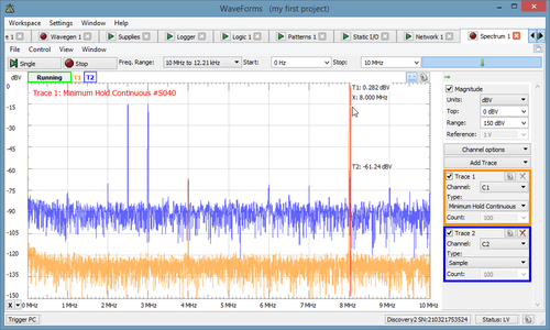
The FFT view plots amplitude against frequency. In other words it shows signals in the frequency domain, as opposed to the time view, which shows signals in the time domain as amplitude against time. It is especially useful for tracking down the cause of noise or distortion in measured signals.
This view contains a subset of Spectrum Analyzer instrument features. To have more options, use this instrument.

The FFT toolbar only shows the important options by default. The down/up arrow in the top left corner shows/hides the other features. This toolbar contains the following:
- Center/Span or Start/Stop: These options adjust the shown frequency range.
- Top: Adjusts the plot top magnitude level.
- Range: Selects the plot amplitude range.
- Units and Reference: See Spectrum Magnitude options.
- Type and Count/Weight: See Spectrum Traces options.
The gear drop-down contains the following options:
- Scale: Selects between Linear and Logarithmic frequency scale.
- Window and Beta: Spectrum Traces options.
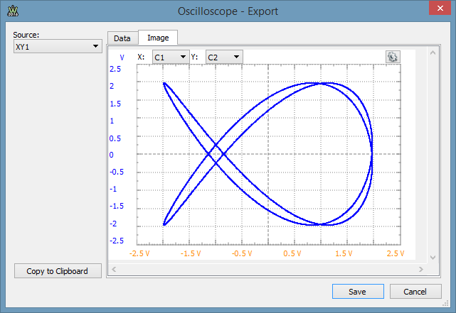
5.2. XY
Using the XY view allows you to plot one channel against another. This plot could be the I-V curve of a component such as a capacitor, inductor, a diode, or a Lissajous figure showing the phase difference between two periodic waveforms. XY view is also capable of more advanced operations, such as plotting a math channel against a reference waveform.
The channels for X and Y representation can be selected on the top side and in the properties button in the top-left corner beside the other plot options.

5.3. Histogram
A histogram is a graphical representation of the voltage distribution in a signal waveform. It plots the distribution of values for each voltage value, with the number of times the signal has a certain voltage value represented as a percentage.
The picture below shows the histogram view of a sine and another signal.
The Auto scale option adjust the scale for each channel separately based on maximum value. With manual scale a common Top level can be specified.

5.4. Data
The Data view displays the acquisition samples and the time stamps.

The column header shows the sample index, the first column shows the time stamp followed by the values for channels.
The selected cells can be copied and pasted to other applications.
5.5. Measurements
The Measurements view shows the list of the selected measurements. The first column in the list shows the channel, the second shows the type, and the third shows the measurement result. See the mouse operations found in the Lists section.
Pressing the Add Default Measurement button opens the Add Measurement window. On the left side is the channel list, and on the right side is a tree view containing the measurement types in groups. Pressing the Add button here (or double-clicking an item) adds it to the measurement list.
The Show menu options allow you to create statistics out of measurements between acquisitions, which can be cleared with the Reset button.


Vertical-axis measurements for each channel:
- Maximum: the absolute largest value.
- Minimum: the absolute smallest value.
- Average: the mean value between maximum and minimum values.
- Peak2Peak: the difference between the extreme maximum and minimum values.
- High: pulse top settled value according to the histogram.
- Low: pulse bottom settled value according to the histogram.
- Middle: the middle value of the pulse between top (High) and bottom (Low) settled values.
- Overshoot: = (Peak to Peak / 2 - Amplitude) / Amplitude.
- Rise Overshoot: = (Maximum - High) / Amplitude.
- Fall Overshoot: = (Minimum - Low) / Amplitude.
- Amplitude: half of the difference between the pulse top (High) and bottom (Low) settled value.
- DC RMS: Direct Current Root Mean Square is the entire power contained within the signal, including AC and DC components.
- AC RMS: Alternating Current Root Mean Square is used to characterize AC signals by subtracting out the DC power, leaving only the AC power component.
Horizontal-axis measurements for each channel:
- Cycles: number of full cycles in visible acquisition data.
- Frequency: frequency of the signal.
- Period: period of the signal.
- PosDuty: positive duty of the signal.
- NegDuty: negative duty of the signal.
- PosWidth: positive pulse-width of the signal.
- NegWidth: negative pulse-width of the signal.
- RiseTime: rise time of the signal.
- FallTime: fall time of the signal.
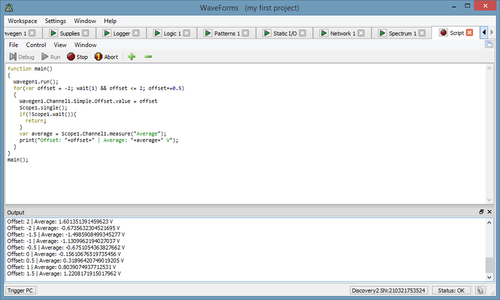
The Add/Custom Channel measurement opens a script editor with an average calculation example script. Here custom measurement involving one channel data can be created. This will be added to the Defined Measurement Custom category list to be used for other channels. See the predefined horizontal measurements that can be opened with Edit as read-only examples.
See Script in Common interfaces. The Locals are Time and Channel object which is the selected channel for the current measurement.
Average calculation:
// initialize a local variable
var value = 0
// loop to access each sample
Channel.data.forEach(function(sample){
// make sum of samples
    value+=sample
})
// divide the sum with the number of samples to get the average
value /= Channel.data.length
// last line of code is the measurement value
value
Accessing other measurements, calculating peak-to-peak value:
Channel.measure("Maximum") - Channel.measure("Maximum")
The Add/Custom Global measurement opens a script editor with an phase calculation example script. Here custom measurement accessing multiple channels can be created. The Local is the instrument object called Scope.
Phase calculation:
// initialize local variables
var sum1 = 0
var sum2 = 0
var sum12 = 0
// for better performance get and use local copy of data array
var d1 = Scope.Channel1.data
var d2 = Scope.Channel2.data
var c = d1.length
for(var i = 0; i < c; i++){
    sum1 += d1[i]*d1[i]
    sum2 += d2[i]*d2[i]
    sum12 += d1[i]*d2[i]
}
sum1 /= c
sum2 /= c
sum12 /= c
// last line of code is the measurement value
Math.acos(sum12/Math.sqrt(sum1*sum2))*180/Math.PI
Accessing other measurements, calculating gain in dB:
Math.log(Scope.Channel1.measure("Amplitude")/Scope.Channel2.measure("Amplitude"))/Math.LN10
The Edit opens the script editor for custom measurements. The predefined Vertical and Horizontal measurements for performance reason are hard-coded and some are shown as read-only example scripts in the editor.
5.6. Logging
See Logging in Common Interfaces.
The script allows custom saving of data, logging, or processed information. The Locals are the instrument object called Scope. Index and Maximum are the values shown above the script.
// local variable
var ch = Scope.Channel1
// condition for saving, average measurement to be less than 5 V
if(ch.measure("Average")<5)
{
    // instantiate file object for acquisition and write channel data
    File("C:/temp/acq"+Index+".csv").write(ch.data)
    // file file for measurements
    var filem = File("C:/temp/measure.csv")
    // in case file does not exists
    if(!filem.exist())
    {
        // write (erasing earlier content) the header line
        filem.writeLine("Time,Average,Peak2Peak")
    }
    // append line with measurement we want to save
    var textm = Date()+","+ch.measure("Average")+","+ch.measure("Peak2Peak")
    filem.appendLine(textm)
    // increment Index
    Index++
}
5.7. X Cursors
The X Cursors show cursor information in table view. See Cursors for more information.
This table shows additional information to cursor tooltips: the 1 / delta x frequency, delta y vertical difference, and delta y / delta x.

5.8. Y Cursors
The Y Cursors show cursor information in table view. See Cursors.
6. Export
See Export in Common Interfaces.
Waveform Generator
The Arbitrary Waveform Generator (or Wavegen) generates electronic waveforms. The waveforms can be either repetitive or single-shot. Different triggering sources can be used: internal (from other devices) or external.
The resulting waveforms can be input into a device being tested and analyzed with the Oscilloscope as they progress through the device. This is useful for confirming the proper operation of the device or pinpointing a fault in the device.
The main window has three areas: the control toolbar at the top, the configuration form(s) on the left side, and the signal preview plot(s) on the right side.

1. Menu
See Menu in Common Interfaces.
1.1. Edit
The Edit menu lets you copy or swap the channels configurations.
2. Control
Run All / Stop All button: starts or stops the selected signal generators.
Channels: selects the channel(s) to be controlled. For every channel you select, a configuration form and a signal preview plot are displayed.
- Channel 1 is Waveform Generator channel 1.
- Channel 2 is Waveform Generator channel 2.
- Channel 3* is the Positive Power Supply (VP+)
- Channel 4* is the Negative Power Supply (VP-)
* Available on Electronics Explorer board.
Synchronization Mode:
- In No synchronization mode, no synchronization parameters are available.
- In Independent mode, the channels are working independently. The trigger-wait-run-repeat settings can be independently configured for each channel. If you modify the settings of a channel, its signal generation starts over from the beginning and synchronization with the other channels is lost.
- In Synchronized mode, the trigger-wait-run-repeat settings are the same for all selected channels within the same instrument instance. Modifying the settings of one of the channels causes both to be restarted. A run time value other than continuous should be used to periodically resynchronize the channels. This has to be done because the actual frequencies might be approximates of the desired values and small errors accumulate until, after several cycles, the channel's phase will slide.
- The Auto synchronization mode is similar to the Synchronized mode where run time is automatically adjusted to the longest period from all channel's settings (depending on signal frequency, sweep/damp time, or AM/FM modulator frequency).
3. Preview
For every channel you select, a signal preview plot is displayed.
The plot options menu on the top-right edge (next to common plot options) contains controls to scale the plot waveforms. Having the Scale option in Full mode allows manual adjustment of time. The vertical scaling in Manual mode can be adjusted as well.
A horizontal left-button mouse drag on the plot changes the start position, and a right-button mouse drag changes the horizontal domain of the preview. A vertical left-button mouse drag on the left/right side changes the modulator/voltage position, and a right-button mouse drag changes the vertical range of the preview.
The actual output might differ from the preview depending on external load, especially at high frequencies.
4. Channel
Run/Stop button: starts/stops the signal generation for the selected channel. The waveform generator channel can be started individually.
Enable button: enables or disables the output.
The channel options allows you to select:
- Idle output: selects the output while not running (Waiting, Ready, Stopped, or Done states).
- Initial: The idle output voltage level has the initial waveform value of the current configuration. This depends on the selected signal type, Offset, Amplitude, and Amplitude Modulator configuration.
- Offset: The idle output is the configured Offset level.
- Disabled *: The idle output is disabled. Channel 1 and 2, outputs 0 Volts. Channel 3 (Positive Power Supply) and Channel 4 (Negative Power Supply), having 1 kOhm resistor to GND and diode.
- Supply*: Selects between voltage and current waveform generator.
- Limitation*: Specifies the current or voltage limitation.
* Available on Electronics Explorer board

5. Configuration Modes
For every channel you select, a configuration mode will be displayed. The custom and play waveforms are shared between the channels and configuration modes.
5.1. Simple
The Simple configuration mode for a simple standard signal configuration.

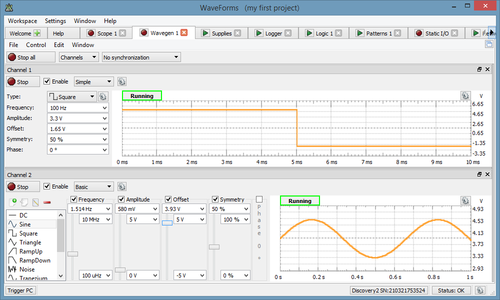
Type represents the standard signal types: DC, Sine, Square, Triangle, Ramp-Up, Ramp-Down, Noise, Trapezium, and Sine-Power. Under the options menu, a Custom waveform can be created and file imported as pattern or play data.
For the Noise signal, the Frequency represents the DAC update rate, and the Symmetry and Phase parameters are disabled.
The Sine-Power signal is a sine signal where the power attribute is 0. For higher power attributes, the waveform tends to have square shape. The function for the power attribute is the following: if (power > 0) = Sin(x) ( 100 / (100-power) ) if (power < 0) = Sin(x) ( (100+power) / 100 )
Frequency, Amplitude, Offset, Symmetry, and Phase allow you to modify signal parameters.
Trigger, Wait, Run, and Repeat settings let you generate burst signals. See States for more information.
5.2. Basic
The Basic configuration mode for standard signal configuration.

Signal icons represent the standard signal type.
Frequency, Amplitude, Offset, Symmetry, and Phase sliders let you easily modify signal values between the maximum and minimum limits. These limits can be adjusted using the combo boxes at the top and bottom of the sliders.
Trigger, Wait, Run, and Repeat settings let you generate burst signals. See States for more information.
5.3. Custom

New button lets you create and edit a new custom waveform. See Editor for more information.
Import button lets you load a waveform from file. See Import file for more information.
Edit button lets you edit the currently selected signal.
Remove button lets you remove the selected or all signals.
Frequency, Sample Rate, Amplitude, Offset, and Phase let you modify the signal parameters.
Trigger, Wait, Run, and Repeat settings let you generate burst signals. See States for more information.
5.4. Sweep
Select Sweep configuration mode for easy setup of sweep and damp signals.

The Sweep and Damp checkboxes enable or disable these modes.
In sweep mode, the signal frequency changes linearly from the first value to the second in the specified time.
In damp mode, the signal amplitude changes linearly from the first level to the second in the specified time.
Type can be a standard or custom. Using the options menu after the signal type, custom signals can be generated or imported from a file. These are added to the type list.
Frequency, Amplitude, Offset, Symmetry, and Phase let you modify signal parameters.
Trigger, Wait, Run, and Repeat settings let you generate burst signals. See States for more information.
5.5. Advanced
Select the Advanced configuration mode for setting complex configurations.

Trigger, Wait, Run, and Repeat settings let you generate burst signals. See States for more information.
Carrier, FM, and AM signals are configured in separate columns.
Type can be a standard or custom. Using the options menu after the signal type, custom signals can be generated or imported from a file. These are added to the type list.
Configurations consist of:
- Type: type of signals includes standard types or custom signals that you define or load. *
- Frequency: adjusts the generated waveform period. Noise signal represents the DAC update rate.
- Amplitude: shows the amplitude for the Carrier signal.
- Index: expresses the modulation index for FM and AM as a percentage.
- Offset: for carrier, adjust the offset in volt units. The modulation offset is expressed as a percentage for modulators.
- Symmetry: is expressed as a percentage.
- Phase: is expressed in degrees.
* With Electronics Explorer board for each channel only one of AM and FM can be custom signal type at a time.
6. States
See Generator States and Idle output for more information.
Using the (Trigger), Wait, Run, and Repeat settings, burst signals can be generated.
- Trigger: specifies the trigger event for the waveform generator channel.
- Wait: specifies how much time to wait before starting the signal generation.
- Run: specifies how long signal generation occurs. The Continuous option causes the signal generator to run continuously.
- Repeat: specifies how many times the (trigger)-wait-run cycle will be repeated. The Infinite option is similar to the Continuous option.
- Repeat Trigger: selects the repeat cycle to include the Trigger in Wait-Run cycle or not.
The following screenshot shows a burst signal.

7. Editor
The Editor lets you easily create arbitrary signal shapes as well as custom carrier signals and modulators.
To launch the Custom editor from the Custom, Sweep, or Advanced configuration form, select the New signal option or select Edit for an existing custom signal.

This lets you generate signals from mathematical functions.
- Name: lets you specify or modify the custom waveform name
- Samples: lets you specify the number of samples. It is useful to create a waveform with a few samples, like steps. The custom waveform will be stretched to fill the available device buffer.
- X from and to: lets you specify the X variable value range used in mathematical function.
- Enter Function: You can type the custom function in this text box. If the entered function is valid, the resulting number for one sample is displayed, otherwise the error description is listed. See Script in Common interfaces. The local variable is X for which the function is called to generate each data sample.
- Normalize: when checked the data will be normalized automatically after Generate.
- Generate: will generate the given function.
- Stretch vertically on the top of the plot will normalize the values between -1 and +1, -100% and +100%.
- Undo / Redo lets you undo/redo the last changes.
- Sample can be edited in the data tab on the right side.
Click OK to save the last valid function. Click Cancel to use the function saved before the editor was opened.
Example functions:
- Math.sin(2*Math.PI*X)+Math.cos(4*Math.PI*X)
- Math.random()*2-1
8. Import
To import a data file into the Custom, Sweep, or Advanced configuration form, select Import and then select File.

Browse button opens a dialog box where you can select a different file to load.
In case the import does not detect the file coding properly, adjust the options in Format group to specify the:
- Skip heading: lines that do not import to data, usually comments or information.
- Column header: check to use a row as column names.
- Column count: specifies the number of data columns in the file.
- Row count: specifies the number of data row in the file.
- List separator
The import group contains the following parameters:
- Column: If the file contains several columns of data, select the one to use.
- First/Count: Specifies the first and the number of sample index to import.
- Offset/Amplitude: Specifies the waveform scale. In case this range is supported by the device, it will be applied when selecting this waveform.
- Samples rate/Frequency: Specifies the rate of the waveform.
Plot area shows the selected data range.
Power Supplies
The power supply interface is different for devices.
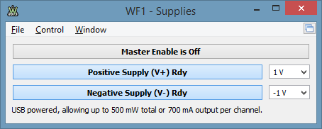
Analog Discovery
This instrument allows you to enable the device power supplies. See Power Supplies for more information.

- Master Enable is ON/OFF button: the master ON/OFF switch for the power supplies.
- Positive/Negative Supply button: the enable switches for each supply.
- RDY is shown when the supply is enabled but the master switch is OFF.
- ON is shown when the master switch is on and the supply is also enabled.
- OFF is shown when the supply is not enabled.
- Power progress bar: shows the consumption of the two power supplies, from zero up to the maximum allowed level.
See Menu in Common Interfaces.
Analog Discovery 2
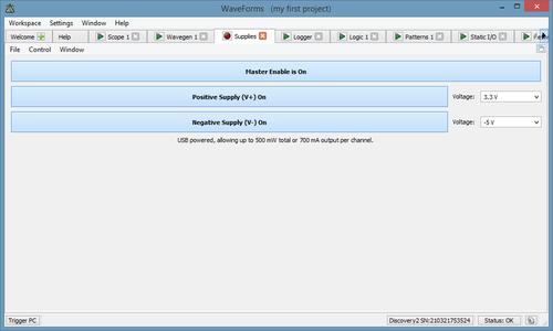
This instrument allows you to enable the device power supplies. See Power Supplies for more information.
- Master Enable is ON/OFF button: the master ON/OFF switch for the power supplies.
- Positive/Negative Supply button: the enable switches for each supply.
- RDY is shown when the supply is enabled but the master switch is OFF.
- ON is shown when the master switch is on and the supply is also enabled.
- OFF is shown when the supply is not enabled.
- Voltage fields: let you adjust values for the power supplies by either selecting a value from combo box, or typing it in.
See Menu in Common Interfaces.
Electronics Explorer
This instrument has two main areas: the control area and the plot window.
The control area contains power supplies with adjustable voltage and current.

See Menu in Common Interfaces.
The control area lets you adjust the settings for the various voltmeters and power supplies.
- Master Enable: the master ON/OFF switch for the power supplies and reference voltages.
- On/Off: are enable switches for each supply.
- Voltage and current fields: let you adjust values for the power supplies by either selecting a value from combo box, or typing it in. Below the adjustment fields the voltage/current reading is shown.
See Meter about the other features.
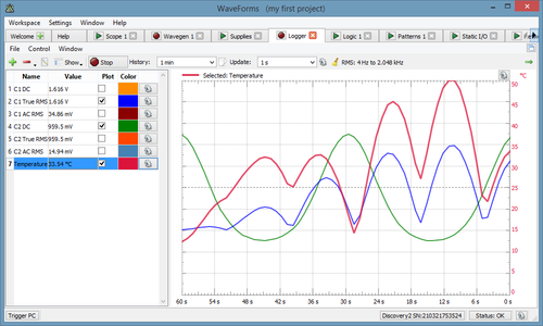
Data Logger
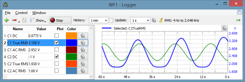
The Data Logger uses the oscilloscope channels. When the Logger is running, it takes control over the two physical oscilloscope channels and the Oscilloscope instrument state is “busy”. Similarly, when the Oscilloscope is started, the Logger is stopped. The oscilloscope sweeps are windowed and DC, AC, and DC RMS values calculated. For the True RMS value, the same acquisition is used as for the DC voltage, and the value is calculated with the formula Sqrt( sum( xi ^ 2 ) / N ). The AC RMS value is calculated with the formula Sqrt( sum( (xi - dc) ^ 2 ) / N ).
1. Plot
The history plot has the following components:
- Add: opens a window. Select an item from the list and press the Add button (or double-click) to add it to the plot list. Using the function field, a custom mathematic channel can be created.
- Remove the selected item(s) from the list.
- Edit the currently selected list item.
- Show: enables or disables columns displaying the minimum and maximum levels from the history plot.
- History: specifies the time span for the plot. Under the history options, update rate and the number of samples can be specified.
- Clear: clear the history plot.
For each channel, the color and scaling option can be specified: auto scaling based on the extremes from the plot history or manually specified offset and range.
See Script in Common interfaces. The local variables are the elementary logger channels, which vary depending on the device.
Example functions:
- C1DC-C2DC
- 25 + C1DC / 0.47
2. Export
See Export in Common Interfaces.
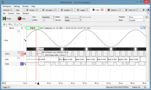
Logic Analyzer
The Logic Analyzer allows acquisition and visualization of digital inputs.
It is possible to configure the information being visualized: to choose which signals to visualize, to group signals in buses, to configure protocol interpreters, and to visualize them in a specific order.

1. Menu
See Menu in Common Interfaces.
1.1. View
- Data: opens/closes the Data view.
- Logging: opens/closes Logging tool.
2. Control

The acquisition bar contains the following:
- Single: starts a single acquisition.
- Run/Stop button: starts repeated, continuous, or stream acquisition (see Run mode below). While the acquisition is in progress, the Run button becomes the Stop button.
- Buffer: The performed acquisitions are stored in the PC buffer in time order. This makes it easy to review a series of repeated acquisitions. The new acquisitions are stored after the currently selected buffer position. If you change the position in the buffer and start a new acquisition, the positions after the selected one will be lost.
- Run: The options in Run mode select the action of the Run button and are the following:
- Repeated: the Run button starts repeated acquisitions.
- Scan Screen: scan acquisition where the sampled data is drawn from left to right. When the right corner is reached, the signal curve plot continues from the left.
- Scan Shift: similar to the screen mode, but when the signal plot reaches the right corner, the curve plot slides to the left.
- Stream: allows capturing a large number of samples at lower rates. In this mode, the samples are streamed trough the USB limiting the rate, depending on the system and other connected devices, at about 1M samples/sec. The scan modes (Screen and Shift) are available when the time-base is greater than a 1 second span, 100 ms/division.
- Mode: The three trigger modes are:
- Normal: the acquisition is triggered only on the specified condition.
- Auto: when the trigger condition does not appear in approximately two seconds, the acquisition is started automatically. In repeated acquisition mode, when the instrument switches to auto trigger, the next acquisitions are made without waiting again to time-out while a trigger event does not occur and the configuration is not changed. When a new trigger event occurs, or the configuration is changed, the current acquisition will be finished and the next one will wait for the trigger again. It is also the best mode to use if you are looking at many signals and do not want to bother setting the trigger each time.
- None: the acquisition is started without a trigger.
- Source: select trigger source between Analyzer trigger condition on pins, other device instrument, or external trigger signals.
- Trigger: shows the trigger configuration.
- Position: adjusts the horizontal trigger position.
- Base: adjusts the time base.
- Gear: opens a menu with the following options:
- Position as division: selects the unit of the position parameter, division, or seconds.
- Range Mode: selects the display mode for time base (per division, plus-minus, and full).
- Rate: adjusts the sample rate.
- Samples: adjust the number of samples to acquire.
- Clock: select internal or external clock source for Logic Analyzer (available on Electronics Explorer).
- Noise: selects to acquire noise samples in half of the buffer.
- Buffers: adjusts the number of PC buffers.
- Update: this specifies the time period at which the application will check the oscilloscope device status and read the acquired data in repeated Run mode. Increase the time to reduce the update rate.
3. Signal Grid

The Signals Grid allows you to customize the display of the signals that you are interested in. See the operations found in the Lists section.
The grid menu contains the following options:
- Add: It is possible to add signals, define, and add a bus or interpreter. One or more signals can be selected and added at a time.


The Bus, SPI, I2C, and UART menus open the corresponding property editor, and after configuring them, it will be added to the grid.
- Remove: It is possible to remove the selected items or the entire list.

- Edit: Under the Edit menu, the following operation can be performed:

- Property: Opens the properties editor for the currently selected item.
The grid columns are as follows:
- Height: the row height can be changed in the first column.
- Expand/Collapse: each bus and interpreter can be individually expanded or collapsed.
- Edit: clicking on the edit icon of a signal, bus, or interpreter row opens the editor.
- IO: Shows the device digital IO pin number. Multiple used signals are marked with star (ex: *3). The not defined signals are noted with ND.
- Trigger: allows you to configure the trigger condition for the Logic Analyzer pins. In this column, a left or right mouse-click opens a drop-down where the trigger condition can be selected. When multiple rows are selected, a right-click sets the trigger for all the selected pins.
The overall trigger condition is built by AND-ing all level conditions together with the result of OR between edge conditions of each pin. The following trigger conditions are possible for each pin:
 Don't Care: not used in trigger condition.

 Low: low logic level.

 High: high logic level.

 Rising Edge: signal transition from low to high level.

 Falling Edge: signal transition from high to low level.

 Any Edge: any signal transition.

The grid context menu opens on mouse right-click. This contains similar buttons as the grid toolbar's Add, Remove, and Edit menus.

The waveform area is divided in three sections: top, bottom, and center.
On the bottom area, the time position can be adjusted by horizontal left mouse button drag and the time base by right mouse button drag.
- Top Area: On the top of the waveform area, the following information is shown: the state of the logic, and viewed acquisition information: number of samples, rate, and capture time. See Acquisition States for more information.
- Bottom Area: On the bottom section, the major time grids are displayed.
- Center Area: This area is used to display rows containing the graphical visualization of waveforms.
3.1. HotTrack
See HotTrack in Common Interfaces.
When the mouse cursor position is in a signal row, it will place a vertical cursor along with two more towards the right, measuring the pulse-width and period. Otherwise, it will place one vertical cursor showing the time position and the waveform's level at the intersections with the vertical cursor.

3.2. Cursors
The Cursors are available for main time view. See Cursors.
The Cursor's drop-down menu contains adjustment controls for the position, reference cursor, delta x value, and remove button.
4. Property Editor
The property editor can be opened for the selected signal, bus, or interpreter under the grid toolbar edit menu.
4.1. Signal

In the signal property editor, the name can be specified and the device pin changed.
4.2. Bus

In the bus property editor, the following can be configured:
- Name: edit the displayed name of the bus.
- Left list: shows the available signals.
- Right list: shows the selected bus signals. The signals can be added or removed with the left/right arrow keys or a mouse drag and drop.
- Enable: selects the optional enable pin and active polarity.
- Clock: selects the optional clock pin and sampling edge.
- Format: selects the values format of the bus.
- Binary values are displayed with “b” leading character.
- Decimal
- Hexadecimal values are displayed with “h” leading character.
- Vector values are displayed with “v” leading character. Vector value is the raw binary value without index.
- Signed
- One's complement
- Two's complement
- Endianness: selects between little and big endian, least significant bit (LSB), first or most significant bit (MSB) first.
- LSB/MSB: selects the values for first and last indices, LSB, and MSB. The index values can be set so that the index remains within the -32 and +31 range.
4.3. SPI

SPI interpreter lets you define a synchronous serial data link with the following options:
- Select: optional slave or chip select signal with low or high active level.
- Clock: is the serial clock with data sampling on rising or falling edge.
- Data: is the serial data signal (MOSI or MISO) with least or most significant bit first shifting.
- Bits: the number of data bits in a transmission word.
- Format: allows selecting the display mode of the value in binary, decimal, or hexadecimal formats.
- Binary values are displayed with “b” leading character.
- Decimal
- Hexadecimal values are displayed with “h” leading character.
- Vector values are displayed with “v” leading character. Vector value is the raw binary value without index.
- Sign and Magnitude
- Ones' complement
- Two's complement
- Leading: skips the given number of starting bits in value calculation.
- Ending: skips the given number of ending bits in value calculation.
4.4. I2C

For I2C or Two Wire Interface interpreter, the clock and data signals can be selected.
4.5. UART

The UART interpreter for asynchronous serial protocols lets you select:
- Data: the data signal.
- Bits: the number of data bits in a transmission word.
- Parity: selects between Odd, Even, Mark (High), and Space (Low) parity modes.
- Baud rate: allows specifying the speed or bits per second of the line.
5. Views
5.1. Data
The Data view displays the data samples.

The column header shows the sample index, the first column shows the time stamp, followed by the values of the added channel's components.
5.2. Logging
See Logging in Common Interfaces.
The script allows custom saving of data or processed information. The Locals are the instrument object called Logic. Index and Maximum are the values shown above the script.
// condition for saving, DIO0 to exists
if('DIO0' in Logic.Channels){
    // instantiate file object for acquisition
    var file = File("C:/temp/dio0_"+Index+".csv")
    var data = Logic.Channels.DIO0.data
    // write data to file
    file.write(data)
    // increment Index
    Index++
}
5.3. Cursors
The X Cursors show cursor information in table view. See Cursors.

6. Export
See Export in Common Interfaces.
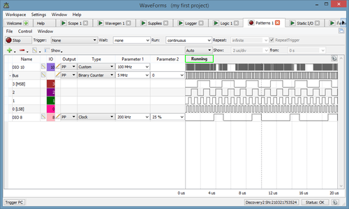
Digital Pattern Generator
The Digital Pattern Generator (Patterns) lets you define the output on the digital lines, using standard types or user-defined types.
When a line is used by the Static I/O as an output element (Slider, Button, or Switch), this has priority over the signal configuration in Patterns.

1. Menu
See Menu in Common Interfaces.
2. Control

Run/Stop button: starts/stops the signal generation.
Trigger, Wait, Run, and Repeat settings let you generate burst signals. See States for more information.
3. Signals Grid

The Signals Grid allows you to customize the display of the signals that you are interested in.
The grid menu contains the following options:
- Add: It is possible to add signals, define, and add a bus. One or more signals can be selected and added at a time.

The Bus menus open the corresponding property editor and after configuring them, it will be added to the grid.
- Remove: It is possible to remove the selected items or clear the entire list.
- Edit: Under the Edit menu, the following operations can be performed:

- Properties: Opens the properties editor for the last selected item.
- Parameters: Opens the parameter editor for the last selected item.
- Show: Under the Show menu, the visibility of grid columns can be selected.
The grid columns are as follows:
- Height: the row height can be changed in the first column.
- Expand/Collapse: each bus can be individually expanded or collapsed.
- Name: shows the signal or bus name.
- Edit: clicking on the edit icon of a signal or bus row opens the editor.
- DIO: shows the device digital IO pin number.
- Parameter: clicking on the edit icon of a signal or bus row opens the parameter editor.
- Type: selects the type (constant, clock, pulse, random, custom, etc.) of signal or bus.
- Output: by clicking on this column, a combo box lets you select the desired output for the corresponding signal or bus.
- Idle: selects the output for the idle state when the generator is not running (Config, Armed, Done, Stopped, or Wait state).
- Parameter #: adjusts the parameter values for the selected signal or bus. The values can be adjusted between the minimum and maximum values selected in the parameter editor.
The grid context menu opens on mouse right-click. This contains similar buttons as the grid toolbar's Add, Remove, and Edit menus. The difference is that instead of signal, bus, or interpreter addition, insert will be performed above the last selected row.

The waveform area is divided into three sections: top, bottom, and center.
On the bottom area, the time position can be adjusted by a horizontal left mouse button drag while the time base can be adjusted by a right mouse button drag.
- Top Area: In the top-left corner, the status label shows the state of the logic patterns. See Generator States for more information.
- Bottom Area: On the bottom section, the major time grids are displayed.
- Center Area: This area is used to display rows containing the graphical visualization of waveforms.
4. Property Editor
The property editor can be opened for the selected signal, bus, or interpreter under the grid toolbar edit menu.
4.1. Signal
In the signal property editor, the name can be specified and the device pin changed.
4.2. Bus

In the bus property editor, the following can be configured:
- Name: edit the displayed name of the bus.
- Available: shows the available signals.
- Selected: shows the selected bus signals. The signals can be added or removed with the left/right arrow keys or a mouse drag and drop. The order of the bus signals can be changed with up/down arrow keys or with a mouse drag and drop.
- Format: selects the values format of the bus.
- Binary values are displayed with “b” leading character.
- Decimal
- Hexadecimal values are displayed with “h” leading character.
- Vector values are displayed with “v” leading character. Vector value is the raw binary value without index.
- Sign and Magnitude
- One's complement
- Two's complement
- Endianness: selects between little and big endian, least significant bit (LSB) first, or most significant bit (MSB) first.
- LSB/MSB: selects the values for first and last indices, LSB, and MSB. The index values can be set so that the index remains within the -32 and +31 range.
5. Parameter Editor
The parameter editor can be opened for the selected signal or bus under the grid toolbar's edit menu, under the context menu, or by double-clicking your mouse on the row.
5.1. Parameters

The type, output, and idle parameters have dedicated columns in the signal definition grid. For the other parameters, a minimum and maximum value can be specified and linearly changed using the track bar.
The Idle parameter lets you select the signal or bus output while not running.
The output type determines the output behavior of the signals and buses. For OD and OS signals, use external pull-up or pull-down resistors. The output types are:
- PP – Push Pull: The allowed values are 0 and 1.
- OD – Open Drain: The allowed values are 0 and Z. The bus value is computed by treating Z as 1.
- OS – Open Source: The allowed values are Z and 1. The bus value is computed by treating Z as 0.
- TS – Three State: The allowed values are 0, 1, and Z. The bus values that contain only 0s and 1s are shown as normal numbers. A question mark is displayed for values that contain Z in at least one of the bus signals.
The possible parameters for different types are the following:
- Constant: By default, a newly added signal or bus is a constant with value Z.
- Output lets you select between PP, OS, OD, and TS.
- Idle lets you select the output value while not running.
- Constant lets you specify the signal(s) value.
- Clock: The parameters used to define a clock signal:
- Output lets you select between PP, OS, and OD.
- Idle lets you select the output value while not running.
- Frequency lets you specify the clock frequency expressed in Hz. The maximum clock frequency is half of the digital base frequency.
- Duty lets you adjust the duty factor between 0% and 100%.
- Phase lets you adjust the clock phase between 0 and 360 degrees.
- Pulse: The initial values for divider and counter specify the initially loaded values, initial delay, when entering in Running state. The Divider specifies the clock division. This rate will be the step for the counter. When entering Running state, the initial divider value specified with is loaded. When this expires, the value specified by divider will be loaded upon each expiration. When the counter initial value expires, the Low and High values are loaded upon further expiration. On counter expiration, the level is toggled and this directs the low or high value loading. In case one of these is zero, the level is not toggled. The parameters used to define a pulse signal:
- Output lets you select between PP, OS, and OD.
- Idle lets you select the output value while not running.
- Start lets you select the pulse to start low or high.
- Low/High lets you adjust the low/high counter values.
- Init lets you adjust the initial counter value. Zero value sets the counter to a low or high value, depending on start parameter.
- Divider lets you adjust the divider value. The base frequency (100 MHz) will be divided by this value for the counter.
- Init lets you adjust the initial divider value.
- Random: The random values are generated on the device. It is not possible to show a preview for this type. To see the output, use the Logic Analyzer instrument or generate custom/random data.
- Output lets you select between PP, OS, OD, and TS. In TS output, the result probability for output levels are the following: Z 50%, 0-low 25% and 1-high 25%.
- Idle lets you select the output value while not running.
- Frequency lets you specify the random output update frequency.
- Number:
- Output lets you select between PP, OS, OD, and TS. In TS mode, the available device buffer size is half the one for other modes.
- Idle lets you select the output value while not running.
- Frequency lets you specify the sample update frequency.
- Number: Using this type, the bus values will be generated as a constant value.
- Output lets you select between PP, OS, and OD.
- Idle lets you select the output value while not running.
- Number lets you specify the bus constant value.
- Binary/Gray/Johnson Counter: Using these types, the bus values will be generated as Binary/Gray/Johnson counter values.
- Output lets you select between PP, OS, and OD.
- Idle lets you select the output value while not running.
- Frequency lets you specify the bus value change rate. For example, at 1 kHz the binary counter will increment every 1ms.
- Number lets you select the counter start value for binary and Gray counters. A Johnson counter will always start with 0 value.
- Walking 0/1: Using these types, the bus values will be generated as a train of 0 or 1 bits walking left or right.
- Output lets you select between PP, OS, and OD.
- Idle lets you select the output value while not running.
- Frequency lets you specify the bit shift rate.
- Direction lets you select left or right shift direction.
- Length lets you specify the train length of the 0 or 1 bits.
5.2. Custom Plot

The custom plot shows the custom data buffer and allows mouse editing. By pressing a mouse button, the value of the corresponding element in the buffer will be changed depending on the vertical position in the row and on the allowed values. By dragging the mouse, multiple buffer positions can be edited with the same value (all positions between the start and the end of the operation). On a bus waveform, all the signals will be changed to the 0, 1, or Z value. Dragging with the left mouse button and changing the vertical position can change the entered value. Dragging with the right mouse button keeps the initial value.
The Samples allow you to specify the used device sample buffer size. On generation, the buffer is repeated while running.
The Undo and Redo buttons allow you to revert the recent changes.
The Show allows you to select a smaller number of samples than the buffer size starting from the specified value.
5.3. Custom Import
The supported import file types are Comma Separated Values and Tab Delimited Text files.

- File: it shows the opened file path and a new file can be selected with the Browse button. The import options can be adjusted under the menu next to the Browse button.
- First: specifies the first sample position to be imported.
- Count: specifies the number of samples to be imported. This can be set up to the minimum between the number of samples in the file or the device buffer size.
- Plot:
- File column: shows the file column names.
- Rows: the file data plot.
- [#] columns: the checkboxes let you select for which signal file data column to import.
Static Input/Output
The Static Input/Output (Static I/O) instrument allows easy configuration of input and output devices on the digital lines. It is called “static” because the value from the digital lines corresponds directly to the values generated or read by the input and output devices. Once a signal value is set, it remains in that state until a new value is set.

See the Menu Strips in Common Interfaces.
1. Groups
The Static I/O controls the digital signals of the device, which are managed in groups of eight: 31-24, 23-16, 15-8, and 7-0. The number of I/O signals depend on the device.

The group type is selected using the group menu. For each line group, the following types can be set: Bit I/O, Slider, Progress bar, or 7-Segment, which are explained in the sections below.
2. Bit I/O
This group type assigns a specific control for each of the eight signals in the group. This controls include: LED, Button, and Switch, which are explained in the sections below.

2.1. LED
This is an input device, indicating the digital line's state.

2.2. Button
This is both an input and output device, implementing a push button with LED indicator. The button has two states: pressed and released.
The button types select the output for released and pressed states.


2.3. Switch
This is both an input and output device, implementing a push/pull switch with LED indicator.


3. Slider
The slider configures the eight digital lines according to either the value of the slider caret's position or the value entered in the direct value field. The value is used as an eight-bit binary representation, where the highest number digital line is the most significant bit (MSB) and each digital line gets the value of the corresponding bit.

4. Progress Bar
This type implements an input device used in displaying values between 0 and 255 as a progress bar and value display. The digital values of the eight input lines are converted into a value between 0 and 255. The digital lines' binary values are used as bits in a binary representation where the highest number digital line is the most significant bit (MSB).

5. 7-segment
This type implements an input device for displaying a seven-segment digit and a decimal point. Each of the eight digital lines correspond to one of the segments or the decimal point, according to the legend displayed on the right of the digits display.

Network Analyzer
The Network Analyzer is used to analyze transfer functions (the ratio between an output function and an input function). The Bode plot shows the magnitude and phase of the expressed function versus frequency. See Bode plot for more information.
Typical usage of Network Analyzer: the WaveGen 1 output and Oscilloscope Channel 1 input of the device is connected to the filter input, while the Oscilloscope Channel 2 is connected to the filter output, as shown in the picture below.

When the instrument is started, the Scope and WaveGen are stopped and their status shows Busy. The Network Analyzer takes control over the these instruments while running.

The analysis is performed from start to stop frequency in the specified number of steps. For each step, the WaveGen channel is set to a constant frequency and the Oscilloscope performs an acquisition. Using the frequency transformation result from the index corresponding to the current frequency step, the magnitude and phase value is calculated. The magnitude of Channel 1 (filter input) is calculated relative to WaveGen Amplitude, and the magnitude and phase values of the other channels are relative to Channel 1. The magnitude is expressed in decibels with the 20 * Log10 (gain) formula, where 1x gain equals 0 dB and 2 X gain equals ~6 dB. The phase is plotted with the maximum and minimum value as the one specified for the Phase Offset +/- 180° value.
With Channel set to none under WaveGen options, no WaveGen channel is controlled. The Oscilloscope acquisitions are expecting a custom or external frequency sweep signal. The current frequency step is determined by peak frequency component with a magnitude of at least half of the specified WaveGen Amplitude value.
With Reference set to none under Scope Options, the magnitude for each channel is calculated relative to the set WaveGen Amplitude and no phase calculated.
1. Menu
See Menu in Common Interfaces.
1.1. View

2. Control
The control area lets you adjust the settings for the network analysis.

- Single button: starts a single analysis.
- Run/Stop button: starts repeated analysis or stops.
- Scale: selects between linear or logarithmic frequency sweep.
- Start: lets you specify the start frequency.
- Stop: lets you specify the stop frequency.
- Steps: lets you specify the number of steps for the analysis.
3. Channels
3.1. WaveGen


- Offset: lets you specify the offset for the generated signal.
- Amplitude: lets you specify the amplitude of the generated signal.
The gear tool contains the following:
- Channel: selects the WaveGen channel to use. With “none” option, an external or custom sweep generator can be used. In this case, the Network Analyzer detects the peak component between start and stop frequencies.
- Settle: specifies the settle time expressed in seconds. The acquisition is delayed this amount of time in each step after the frequency is changed. This option can be used to reduce the alteration effect of resonant circuits (for instance, a speaker).
- Min Periods: specifies the minimum number of generated sine periods to capture.
3.2. Magnitude

- Units: selects between dB and gain representation of magnitude on Bode plot.
- Top: lets you specify the top of the magnitude plot.
- Range: lets you specify the range of the magnitude plot.
3.3. Phase

- Offset: lets you specify the offset of the phase plot.
- Range: lets you specify the range of the phase plot.
3.4. Add Channel
Saves a channel as a reference to compare with further analysis.
3.5. Channel


- Use as Reference: selects to use Scope Channel 1 as reference for the other channels.
- Offset: lets you specify the offset of the Scope channel.
- Gain: lets you specify the gain of the Scope channel relative to the WaveGen amplitude.
The gear tool contains the following:
- Color: sets the channel waveform color.
- Attenuation: specifies the used probe attenuation.
- Range: lets you specify the range of the Scope channel.
- Export: opens export window with the respective channel data, see Export in Common Interfaces.
- Name: specifies the channel name.
- Label: specifies the channel label.
3.6. Reference


The Reference options contains the following:
- Color: sets the channel waveform color.
- Update: updates reference channel with the selected channel waveform.
- Export: opens export window with the respective channel data, see Export in Common Interfaces.
- Name: specifies the channel name.
- Label: specifies the channel label.
4. Bode Plot
The Bode plot shows the magnitude and phase.
By default, the Channel 1 magnitude is relative to the WaveGen amplitude. The magnitude and phase values of the other channels are relative to channel 1.
The gear tool (in the top-right corner or mouse right-click) contains options for:
- Color: selects the color theme for this plot.
- Plot Width: sets the thickness of the waveform, expressed as points.

4.1. HotTrack
See HotTrack in Common Interfaces.
The corresponding position is marked with a cross on Nichols and Nyquist plots.
4.2. Cursors
See Cursors in Common interfaces.
5. Views
5.1. Time Plot
The time plot shows the oscilloscope acquisition of the last frequency step. This view is used to help adjust the offset and gain of the oscilloscope input channels.

5.2. Nyquist Plot
The Nichols plot is the magnitude and phase plotted in the polar coordinate system.

5.3. Nichols' Plot
The Nichol's plot is the magnitude and phase plotted in the Cartesian coordinate system.

5.4. Cursors
The Cursors show cursor information in table view.
This table shows additional information to cursor tooltips: the 1 / delta x frequency, delta y vertical difference and delta y / delta x.

6. Export
See Export in Common Interfaces.
Spectrum Analyzer
The Spectrum Analyzer instrument measures the magnitude of an input signal versus its frequency.
The Spectrum Analyzer uses the oscilloscope channels to acquire input signals. Because of this, all instruments that use the oscilloscope channels will cease acquisition when the Spectrum Analyzer begins sampling.

1. Menu
See Menu in Common Interfaces.
1.1. View

- Time: opens/closes the Time view.
- Measure: opens/closes the Measurements.
- Components: opens/closes the Components.
- Cursors: opens/closes the Cursors.
2. Control

The control toolbar by default only shows the important options. The down/up arrow in the top left corner shows/hides the other features. This toolbar contains the following:
- Single button: starts a single acquisition.
- Run/Stop button: starts repeated acquisition. While the acquisition is in progress, the Run button becomes the Stop button.
- Freq. Range: The frequency range options selects the operation range of the Spectrum Analyzer. Having the auto option selected, the maximum frequency or sampling rate is determined based on the stop or highest value between start and stop.
- Scale: Selects between Linear and Logarithmic frequency scale.
- Center/Span or Start/Stop: The frequency halfway between the stop and start frequencies is known as the Center frequency. This is the frequency that is in the middle of the display’s frequency axis. The Span parameter specifies the range between the start and stop frequencies. Alternatively, the Start and Stop frequencies can be specified.
- BINs: Adjusts the number of frequency bins.
- Samples: Adjusts the number of time domain and oscilloscope acquisition samples.
- Resolution: Adjusts the frequency resolution bandwidth. The gear drop-down contains the following options:
- Algorithm:
- FFT: Fast Fourier Transform (quick process) expects a number of input samples (always a power of 2). It then outputs half of this number in frequency BINs, linear from 0 to half of the sampling frequency.
- CZT: Bluestein's Chirp-Z Transform expects an arbitrary number of input samples. It then outputs arbitrary number of frequency BINs, linear from the specified start to stop frequencies. This allows resolution to increase by interpolation. It allows smooth adjustment of resolution bandwidth with a flexible number of input samples and output BINs.
- Update: This specifies the time period at which the application will check the oscilloscope device status and read the acquired data. Increase the time to reduce the update rate.
3. Traces
3.1. Magnitude

- Units: Selects the amplitude units:
- Vpeak: Relative to 1V amplitude sine wave.
- Vrms: Relative to 1V RMS (1.41V amplitude) sine wave.
- dBV: dB reference to 1Vrms sine wave power, 20*Log10(Vrms).
- dBu: dB reference to 0.775Vrms sine wave power, 20*Log10(Vrms/0.775).
- dB: dB reference to peak voltage value.
- Top: Adjusts the top amplitude level. The channel's input range with Auto option is configured according to this setting.
- Range: Selects the amplitude range.
- Reference: Adjusts the peak voltage reference for dB unit selection.
3.2. Channel
The options in the drop-down menu allow configuration of each oscilloscope channel as follows: Offset, Range, Attenuation, and Sample Mode; and to configure trigger. Having the Auto option for Range, the range is adjusted based on Magnitude Top value.
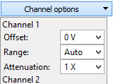
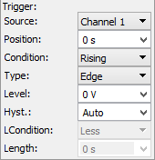
3.3. Trace
The Add Trance drop-down menu contains:
- Add Normal Trace: This adds a trance with default or its last settings.
- Reference: This allows cloning an existing trace settings and data with Hold option, to be used as reference trace.


Up to eight traces can be added. For each trace the following options can be individually configured:
- Channel:The channel option selects the input of the trace, one of the oscilloscope inputs of the connected device, or Hold keeps the trace unchanged/unaffected by the new sweeps.
- Type: Selects one of the following:
- Sample: The trace is updated after each sweep.
- Peak Hold Cont.: Continuous peak hold, keeps the maximum values for each bin from consecutive sweeps.
- Peak Hold: The trace is updated after the specified count of sweeps.
- Min Hold Cont.: Continuously keeps the minimum amplitude values for each bin from consecutive sweeps.
- Min Hold: The trace is updated after the specified count of sweeps.
- Linear RMS Average: The trace is updated after the specified count of sweeps with linear average of Vrms amplitudes.
- Linear dB Average: The trace is updated after the specified count of sweeps with linear average of dB amplitudes.
- Exp. RMS Average: Performs exponential averaging of Vrms amplitudes. It is calculated using the following formula:
- Averagei = Rrms(Sweep)/Weight + Rms (Average)(i-1)*(Weight -1)/Weight
- Exp. dB Average: Performs exponential averaging of Vrms amplitudes. It is calculated using the following formula:
- Averagei = dB(Sweep)/Weight + dB (Average)(i-1)*(Weight -1)/Weight
- Count/Weight: Specifies the count or weight for the selected averaging methods.
The options drop-down contains the following settings:
- Color: sets the channel waveform color.
- Window: Selects the window function:
- Rectangular: Good for closely spaced sine waves and white noise analysis.
- Triangular
- Hamming: Good for closely spaced sine waves.
- Hann(ing): Good for unknown content, narrowband, and combination of sine waves.
- Cosine
- Blackman-Harris
- Flat Top: Reduces resolution but is good in amplitude accuracy.
- Kaiser: See Window Functions for more information.
- Beta: Adjusts the π*α parameter of Kaiser window.
- Export: Opens export window with the respective trace data. See Export in Common Interfaces.
- Name: specifies the channel name.
- Label: specifies the channel label.
4. Plot
The main spectrum plot shows the magnitude versus frequency. About frequency settings see the Control toolbar and Magnitude options.

See Plots in Common Interfaces.
4.1. HotTrack
See HotTrack in Common Interfaces.
Having the mouse cursor in the upper half of the plot, the HotTrack will search and position at a nearby peak. In the lower half of the plot it is not searching for peaks.
4.2. Cursors
See Cursors in Common interfaces.
5. Views
5.1. Time View
The time plot shows the last oscilloscope acquisition. This view is used to help adjusting optimal offset and range for each channel.

5.2. Measurements
The Measurements view shows the list of the selected measurements. The first column in the list shows the channel, the second shows the name, the third shows the measurement value, frequency, and alias frequency for components, along with some other measurements. At the top are Add and Remove and Options drop-down button.
Pressing the Add button opens the Add Measurements window. On the left side is the channel list, and on the right side is a tree view containing the measurement types in groups. Below it is the current value of the measurement and a short description. Pressing the Add button here (or double-clicking an item) adds it to the measurement list.

The measurement options:
- Harmonics: Maximum number of harmonics to search for.
- Alias: Search for high frequency harmonics, above analysis frequency limit, reflected by sampling frequency.
- Excursion: The minimum excursion level needed for a peak to be considered a valid harmonic.
Constant
- ENBW: Normalized equivalent noise bandwidth of window function.
- Resolution: Resolution of bins, bin to bin distance.
- RBW: Resolution bandwidth is calculated from the transform resolution and window bandwidth.
- FS: Full scale is the input range, maximum magnitude of sine wave before clipping.
- DNR: Dynamic range is the ratio, in dB, of the largest to the smallest signals that can be detected.

- Bits: AD Converter bits.
- BINs: Number of frequency bins, selectable from the frequency toolbar.
- Samples: Number of time domain acquisition samples, selectable from the frequency toolbar.
Dynamic
- NF: Noise floor is a root mean square (RMS) of all the bins except the peak signal and its harmonics.
- WoSpur: Worst spur level may or may not be a harmonic of the original signal; DC and bins on the descending slope are excluded.
- SFDR: Spurious free dynamic range is the ratio of the RMS value of the peak signal to the RMS value of the worst spurious signal. Expressed in dBc units, with respect to the actual signal amplitude.
- SFDRFS: Spurious free dynamic range, expressed in dBFS units, with respect to full-scale.
- SNR: Signal to noise ratio, S/N:

Where Vmrsi are all bins except peak signal, its harmonics, and DC. The exceptions are the descending slope bins of the earlier mentioned peaks.
- SNRFS: Signal to noise ratio, expressed in dBFS units, with respect to full-scale.
- THD: Total Harmonic Distortion, S/D

Where Vmrsi are the harmonic peak values.
- SINAD: Signal to noise and distortion, S/(N + D).

Where Vmrsi are all BINs except peak signal and DC, also excluding bins in the descending slopes of these.
- ENOB: Effective number of bits.

Harmonics
- FF: Fundamental frequency and magnitude.
- Nth: Harmonics frequency and magnitude value relative to fundamental frequency. The maximum number of harmonics can be configured in the Measurement options.
5.3. Components
The components view shows the spectral component list for the chosen trace ordered by magnitude. The count parameter sets the number of component to list.

5.4. Cursors
See Cursors.
6. Export
See Export in Common Interfaces.
Script

The Script window allows execution of WaveForms scripts. The scripting language is JavaScript, based on the ECMA Script standard.
From the script code, objects behind the user interface can be accessed. This allows configuration using the interface and automating parts of it with script.
1. Menu
See Menu in Common Interfaces.
2. Control
The control toolbar allows you to debug and execute the script.

- Debug: starts the Qt Script Debugger.
- Run: executes the script.
- Stop: stops debugging or execution. In order for this to work, the code needs to use the instrument.wait() function which returns false when the script or instrument what stopped; or wait() function, which needs to return when this function returns false.
- Abort: forces the execution to interrupt.
- Zoom In/Out: increase or reduce code font size.
3. Output
The output window contains the print() messages and error log.
4. Code
The instrument's object can be accessed from the script and has the most relevant child objects and parameters in the table below.
The instrument parameters are stored in objects with the following properties:
- text: text representation of parameter.
- value: index of discrete setting (like mode: None, Auto, Normal) or value expressed in units.
- preset: list of discrete settings or nice value steps.
wait(seconds): Waits the specified number time expressed in seconds. If the value is 0 or if the argument is missing, then the function is ignored. With negative value, it waits until stopped. Returns false when the script is stopped; otherwise returns true.
print(arg0,arg1,…): Prints the arguments to the Output window.
Device
- .isConnected: is connected to a device
- .name: device name
- .SN: serial number
instrument#: common instrument object
- .single(): single acquisition
- .run(): run instrument
- .stop(): stop instrument
- .wait(): wait for the acquisition to be done or instrument stopped
- .State
- .text instrument states: Disabled, Ready, Done, Stop, Busy, Error, Config, Armed, Trig'd, Running, Auto, Scan, Wait
- .running(): returns true when the instrument is in active state, >= Config
- .Rate.value: refresh rate of the instrument, the device communication rate
- .Time
- .Position.value
- .Base.value
- .Samples.value
- .Rate.value
Scope#
- .measure(name): global measurements
- .Trigger: trigger configuration
- .Mode.text: acquisition mode: Normal, Auto, None
- .Run.text: run-scan mode: Repeated, Screen, Shift
- .Type.text: trigger type: Edge, Pulse, Transition
- .Source.text: trigger source
- .Condition.text: condition: Rising, Falling or Positive, Negative
- .Level.value
- .Hysteresis.value
- .LCondition.value
- .Length.value
- .HoldOff.value
- .Filter.text: sample type to use when looking for trigger condition: Decimate, Average
- .BufferSize.value: PC buffer size
- .Buffer.value: selected PC buffer index
- .Digital.checked: enable or disable digital channels
- .DigitalChannels: digital channels, same as Analyzer#.Channels
- .DigitalTrigger: same as Analyzer#.Trigger
- .channel#: the following properties are available for Math and Ref channels as well:
- .checked: get data array
- .measure(name): Channel measurements: Minimum, Maximum, Average, Peak2Peak, Low, High, Amplitude, Middle, …
- .Offset.value
- .Range.value
- .histogram: gets the histogram array
- .HistogramIndex2Data(index): returns the “voltage” value corresponding to the histogram array index
- .Channel#: real channels
- .Attenuation.value
- .Noise.checked
- .SampleMode.text: sampling mode: Decimate, Average, Min/Max
- .Ref#: reference channels
- .data: set data
- .clone(channel): clone with channel
- .TimeRef: reference channel time
- .Units.text
- .Noise.checked
- .Math#: mathematic channels
- .Operation.text: simple mode operation
- .A: simple mode channel A
- .B: simple mode channel B
- .Custom.checked: enable custom mode
- .Function.text: custom function
- .Units.text
- .Histogram
- .Autoscale.checked
- .Top.value: top of the scale to use when auto-scale is unchecked
.Wavegen#
- .Synchronization.text: synchronization mode: No synchronization, Independent, Synchronized, Auto synchronized
- .States: common synchronization states settings
- .Trigger.text
- .Wait.value
- .Run.value
- .Repeat.value
- .RepeatTrigger.checked
- .Channel#
- .Mode.text: configuration mode: Simple, Basic, …
- .Options
- .IdleOutput.text: idle output value: Offset, Initial, Disabled
- .States: channel states configuration
- .Simple
- .Type.text: waveform type: Sine, Square, …
- .Frequency, Offset, Amplitude, Symmetry, Phase
- .value
- .Basic
- .Type.text
- .Frequency, Offset, Amplitude, Symmetry, Phase
- .value
- .Min.value
- .Max.value
- .Custom
- .Type
- .text
- .set(name,array): set custom waveform data (normalized to +-1) identified by name
- .add(array): add custom waveform, name of waveform is returned
- .Frequency, Offset, Amplitude, Symmetry, Phase
- .value
- .Sweep
- .Type
- .text
- .set(name,array): set custom waveform data (normalized to +-1) identified by name
- .add(array): add custom waveform, name of waveform is returned
- .Offset, Symmetry, Phase
- .value
- .Frequency
- .checked: enable sweeping
- .Start.value: start frequency
- .Stop.value: stop frequency
- .Time.value: sweep time
- .Amplitude
- .checked: enable damping
- .Start.value: start amplitude
- .Stop.value: stop amplitude
- .Time.value: damp time
.Analyzer#
- .Trigger: trigger configuration
- .Mode.text: acquisition mode: Normal, Auto, None
- .Clock.text: clock source: Internal, External
- .Source.text: trigegr source
- .Run.text: run-scan mode: Repeated, Screen, Shift
- .BufferSize.value: PC buffer size
- .Buffer.value: selected PC buffer index
- .Channels
- .channel: channel like: DIO1, Bus1, SPI1
- .name: channel name
- .data: get data array
- .DIO#
- .DIO.value: digital I/O pin index
- .Trigger.text: trigger: Ignore, Rise, Fall, Edge, High, Low
- .Bus#
- .Enable.DIO.value: enable pin
- .Clock.DIO.value: clock pin
- .Active.text: enable active level: Low, High
- .Polarity.text: sampling clock edge: Rising, Falling
- .Format.text
- .Endianness.text
- .MSB.text
- .LSB.text
- .Pin#
- .DIO.value: digital I/O pin index
- .SPI#
- .Select, Clock, Data
- .DIO.value: digital I/O pin index
- .Active.text: select active level: Low, High
- .Sample.text: sampling clock edge: Rising, Falling
- .First.text: data bit order: LSB, MSB
- .Bits.value: word bits
- .Format.text
- .Leading.value: skip leading bits
- .Ending.value: skip ending bits
- .I2C#
- .Clock, Data
- .DIO.value: digital I/O pin index
- .UART#
- .Data
- .DIO.value: digital I/O pin index
- .Bits.value: word bits
- .Parity.text: parity setting: “None”, “Even”, “Odd”, “Mark (High)”, “Space (Low)”
- .Rate.value: baud rate setting
.Patterns#
- .States
- .Trigger.text
- .Wait.value
- .Run.value
- .Repeat.value
- .RepeatTrigger.checked
- .Preview.text: preview mode: Manual, Auto
- .Channels
- .channel: channel like: DIO1, Bus1, SPI1
- .name: channel name
- .data: get data array
- .DIO#
- .DIO.value: digital I/O pin index
- .Bus#
- .Format.text
- .Endianness.text
- .MSB.text
- .LSB.text
- .Pin#
- .DIO.value: digital I/O pin index
.StaticIO
- .Channel#: groups of 8 signals
- .Mode.text: select between: I/Os, Slider, Progress
- .Input.value: input value
- .DIO#: I/Os
- .Input.checked: input value
- .Mode.text: select between: LED, Button, Switch
- .Button.text: select between: 0/1, 1/0, Z/1, 1/Z, Z/0, 0/Z
- .Switch.text: select between: TS, PP, OS, OD
Supplies
- .MasterEnable.checked
- .Output: for Analog Discovery
- .PositiveSupply.Enable.value
- .NegativeSupply.Enable.value
- .Output: for Electronics Explorer
- .PositiveSupply, NegativeSupply
- .Enable.value
- .Voltage.value
- .Current.value
- .DigitalSupply, Refernce1, Reference2
- .Enable.value
- .Voltage.value
- .Input: for Electronics Explorer same as Meter#.Input
Meter
- .Input: for Analog Discovery uses Scope inputs
- .Channel#
- .DC, TrueRMS, ACRMS
- .value
- .Input: for Electronics Explorer
- .PositiveSupply, NegativeSupply, DigitalSupply
- .Voltage.value
- .Current.value
- .Voltmeter#
- .Voltage.value
- .Meters: channels in history list
- .History.value
- .Samples.value
File(path-name): file object constructor
- .exists(): returns true if the file exists; otherwise returns false
- .getName(): returns the file name
- .getPath(): returns the file path
- .getSize(): return file size in bytes
- .isReadOnly(): return true if the file is read-only; otherwise returns false
- .isHidden(): return true if the file is hidden; otherwise returns false
- .getLastModified(): returns the date and time when the file was last modified
- .getCreation(): returns the date and time when the file was created
- .rename(name)
- .copy(path)
- .move(path)
- .deleteFile()
- .read(): read file content as string
- .read(size): reads up to size bytes from the file as string
- .readArray(): reads the entire file as string array, expects values split by comma, white space or new line
- .write(string): write argument as string to file
- .writeLine(string): write argument as string to file followed by a new line
- .append(string): appends argument as string to file
- .appendLine(string): appends argument as string to file
- .readInteger(): read file content as integer (32-bit) array
- .writeInteger([]): write array argument as integer array
- .appendInteger(number): appends argument as integer to file
- .readFloat(): read file content as floating point number (32-bit) array
- .writeFloat([]): write array argument as floating point number array
- .appendInteger(number): appends argument as floating point number to file
- .readDouble(): read file content as double precision floating point number (64-bit) array
- .writeDouble([]): write array argument as double precision floating point number array
- .appendDouble(number): appends argument as double precision floating point number to file
Tool: helper functions
- .question(text): Opens a Yes or No question message box with the given text. Returns true when Yes pressed; otherwise returns false.
- .getText(label, text): Get a string from the user.
- .getNumber(label, value, minimum, maximum, decimal places): Gets a floating point input from the user.
- .getInteger(label, value, minimum, maximum): Gets an integer input from the user.
- .getItem(label, value, items array, current index, editable): Lets the user select an item from a list. Returns the selected text.
- .start(program, argument array, work directory): Starts the program with the given arguments. Returns true on success; otherwise returns false.
5. Examples
The following code starts the waveform generator instrument, performs an oscilloscope acquisition, then computes and prints the average value.
Wavegen1.run()
Scope1.single()
Scope1.wait()
var average = 0
var data = Scope1.Channel1.data
data.forEach(function(sample){
  average += sample
})
average /= data.length
print("Average: "+average+"V")
The following code saves the acquisition sample array to a file.
File("C:/temp/acquisition.csv").write(Scope1.Channel1.data)
The following code sets the trigger source and level of oscilloscope instrument based on user input.
Scope1.Trigger.Source.text = Tool.getItem("Source", Scope1.Trigger.Source.preset, Scope1.Trigger.Source.value)
Scope1.Trigger.Level.value = Tool.getNumber("Level", Scope1.Trigger.Level.value)
The following code creates a custom waveform and sets it to be further used.
wave = Array()
for(var i = 0; i < 10; i++){
  wave.push(0)
  wave.push(i/10)
}
Wavegen1.Channel1.Mode.text = "Custom"
Wavegen1.Channel1.Custom.Type.set("MyWave", wave)
Wavegen1.Channel1.Custom.Type.text = "MyWave"
The following code increases the offset level.
Wavegen1.Channel1.Mode.text = "Simple"
Wavegen1.start()
while(!Tool.question("Are we there yet?")){
  Wavegen1.Channel1.Simple.Offset.value += 0.1
  print("Offset: "+ Wavegen1.Channel1.Simple.Offset.text)
}
The following code sets slider for one Static I/O and increments the value twice a second.
StaticIO.Channel0.Mode.text = "Slider"
for(var i = 0; wait(0.5); i++, i%=256){
  StaticIO.Channel0.Slider.value = i
}
StaticIO.Channel0.Mode.text = "Progress"
SDK and Runtime
The WaveForms installer includes the sdk. The WaveForms SDK is a software development kit for creating custom applications and consists of user manual, examples in Python and C++, and library header file.
The WaveForms installer also includes the WaveForms Runtime. The WaveForms runtime consists of a shared library (dwf) and device support files and is needed for running custom applications.
WaveForms toolkit for LabVIEW
The Digilent WaveForms Toolkit for LabVIEW makes it easy to automate your Digilent instruments with LabVIEW software. This standard API supports Analog Discovery, Analog Discovery II, and the Electronics Explorer, and it includes MSO VIs to set up measurements and acquire data from mixed-signal oscilloscopes, FGEN VIs to output waveforms with the function generator, DIG VIs for reading and writing digital I/O, and PWS VIs for configuring and controlling the power supplies.
A Getting Started with LabVIEW and Analog Discovery 2 guide is provided by National Instruments.